

Probabilistic TSK Fuzzy System in the Simultaneous Learning of Structure Identiflcation and Parameter Optimization
-
摘要: 传统Takagi-Sugeno-Kang (TSK)模糊系统的结构辨识和参数优化往往分阶段进行, 同时模糊规则数需要预先设定, 因此TSK模糊系统的逼近性能和解释性往往不理想.针对此问题, 提出了一种结构辨识和参数优化协同学习的概率TSK模糊系统(Probabilistic TSK fuzzy system, PTSK).首先, PTSK使用概率模型表示模糊回归系统, 将结构辨识和参数优化作为一个整体来考虑.其次, PTSK不借助于专家经验, 使用粒子滤波方法对规则数和前后件参数协同学习, 得到系统全部参数的最优解.实验结果表明, PTSK具有良好的逼近性能, 同时能获得较少的模糊规则数.
-
关键词:
- Takagi-Sugeno-Kang模糊系统 /
- 概率模型 /
- 回归 /
- 粒子滤波
Abstract: Most of existing Takagi-Sugeno-Kang (TSK) fuzzy systems identify their structure and estimate antecedent/consequent parameter of rules in a stepwise manner. In addition, the number of fuzzy rules generally has to be decided manually. Therefore, the performance and interpretability of TSK fuzzy systems are often not satisfactory. In order to overcome these shortcomings, in this paper, a novel probabilistic TSK fuzzy system called probabilistic TSK fuzzy system (PTSK) is constructed from the perspective of probabilistic model. Firstly, PTSK uses a likelihood probability to characterize fuzzy regression tasks, while considering structure identification and parameter optimization as a whole. Secondly, without any prior expert experience, PTSK adopts a particle filter method to simultaneously learn the number of rules and antecedent/consequent parameter of fuzzy rules. According to the experimental results on several datasets, PTSK obtains good approximation performance and a relatively small number of fuzzy rules.-
Key words:
- Takagi-Sugeno-Kang fuzzy system /
- probabilistic model /
- regression /
- particle filter
1) 本文责任编委 许斌 -
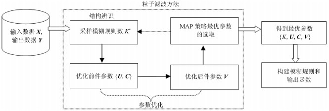
图 1 PTSK结构辨识和参数优化的协同学习示意图
Fig. 1 The diagram of simultaneous learning of structure identiflcation and parameter optimization in PTSK
表 1 聚类法TSK模糊系统中常用的模糊规则前件/后件参数学习方法
Table 1 The common learning methods for the antecedent/consequent parameters in the clustering based TSK fuzzy system
前件参数学习 FCM模糊聚类[5] 优点 获得的空间划分具有模糊性, 算法实现简单 缺点 聚类数需要预先设定 Gustafson-Kessel[13]和Gath-Geva聚类[14] 优点 均使用诱导矩阵识别数据集的结构 缺点 矩阵计算量较大 One-pass聚类[15] 优点 数据集只需要遍历一遍即可完成空间划分, 适用于增量或在线学习模式 缺点 对凸型数据分布识别较差; 且与聚类数有关的参数需要预先设定 后件参数学习 最小二乘法[3, 8] 优点 最常用; 显式地得到后件参数的解析解, 计算简单 缺点 对噪声数据敏感 支持向量回归机[15] 优点 保证参数的全局最优解, 逼近性能较强 缺点 二次规划问题求解的计算量较大 进化计算[4] 优点 模拟自然随机优化算法, 不依赖对象的数学模型 缺点 遗传编码的选择较难解决, 时间复杂度较高 反向传播算法[16] 优点 在小数据集上很快达到局部最优解 缺点 收敛较慢, 不适用于大规模数据集  下载: 导出CSV
表 2 数据集基本信息
Table 2 Basic information of datasets
数据集 规模 维数 abalone 4 177 8 anacalt 4 052 7 autompg6 392 5 autompg8 392 7 bodyfat 252 14 compactiv 8 192 21 concrete 1 030 8 dee 365 6 delta-ail 7 129 5 delta-elv 9 517 6 diabert 43 2 elevators 16 599 18 friedman 1 200 5 gc-s 56 000 6 gc-x 56 000 6 gc-p 56 000 6 housing 506 13 mexihat 2 500 2 mg 1 385 6 mortgage 1 049 15 plastic 1 650 2 pole 14998 26 puma32h 8 192 32 quake 2 178 3 stock 950 9 treasury 1 049 15 wankara 1 609 9 wizmir 1 461 9
下载: 导出CSV
表 3 算法参数设置
Table 3 Parameter setting
算法 参数设置 L2-TSK-FS 模糊规则数$K\in \{{{2}^{2}}, {{3}^{2}}, \cdots, {{11}^{2}}\}$, 尺度参数$h\in \{{{0.2}^{2}}, {{0.4}^{2}}, \cdots, {{2}^{2}}\}$, 模糊指数$m=2$, 正则化参数$C\in\{{{2}^{-4}}, {{2}^{0}}, \cdots, {{2}^{7}}\}$. TSK-IRL-R 适应性函数最小匹配度= 1.5, 种群数= 61, 交叉概率= 0.1, 种群比例=0.2. MOGUL-R 正类样本的匹配度参数= 0.05, 负类样本的允许比例参数= 1.5, 适应性函数最小匹配度= 0.1, 种群数= 15. B-ZTSK-FS 模糊规则数$K\in \{{{2}^{2}}, {{3}^{2}}, \cdots, {{11}^{2}}\}$, 尺度参数$h\in \{{{0.2}^{2}}, {{0.4}^{2}}, \cdots, {{2}^{2}}\}$, 模糊指数$m=2$, 狄利克雷参数= 1 000. WM 标签数= 5. ENSEMBLE 隐层数= 2, 隐结点数= 15, 学习系数= 0.15, 动量系数= 0.1, 集成方法类型: BEM, 网络数= 10. PSVR 正则化参数$C\in \{{{10}^{-3}}, {{10}^{-2}}, \cdots, {{10}^{3}}\}$, 高斯核核参$\sigma \in\{{{10}^{-3}}, {{10}^{-2}}, \cdots, {{10}^{3}}\}$. PTSK 模糊指数$m=2$, 最大迭代次数${10}^{3}$, 阈值$\varepsilon =10^{-3}$, 收敛阈值$miter=50$, 稀疏参数$\beta \in \{1, 2, \cdots, 8\}$, 粒子数$P=10$.
下载: 导出CSV
表 4 8 种算法在 28 个数据集上的 MSE (标准差) 比较
Table 4 MSE (Standard deviation) comparison of 8 algorithms on 28 datasets
数据集 ENSEMBLE-R PSVR WM-R MOGUL-R TSK-IRL-R L2-TSK-FS B-ZTSK-FS PTSK mexihat 0.0205 0.0222 0.0219 0.0207 0.0231 0.0226 0.0239 $ \bf{0.0204}$ 1.004$\times {{10}^{-3}}$ 1.023$\times {{10}^{-3}}$ 1.011$\times {{10}^{-3}}$ 1.025$\times {{10}^{-3}}$ 1.017$\times {{10}^{-3}}$ 1.003$\times {{10}^{-3}}$ 1.020$\times {{10}^{-3}}$ 1.001$\times {{10}^{-3}}$ abalone 4.1738 5.0107 6.6225 4.7323 5.8258 5.1987 4.1186 $ \bf{ 4.0810}$ 0.383 0.376 0.301 0.273 0.326 0.298 0.213 0.196 anacalt 0.0531 0.0478 0.0595 0.0521 0.0829 0.0542 0.0496 $ \bf{0.0435 }$ 1.452$\times {{10}^{-3}}$ 1.023$\times {{10}^{-3}}$ 4.520$\times {{10}^{-3}}$ 1.102$\times {{10}^{-3}}$ 4.239$\times {{10}^{-3}}$ 2.358$\times {{10}^{-3}}$ 2.102$\times {{10}^{-3}}$ 1.404$\times {{10}^{-3}}$ autompg6 11.8797 11.8827 13.3320 14.1473 $\bf{ 8.2574}$ 13.6705 12.3298 11.0676 4.831 2.681 1.821 8.553 1.325 1.964 1.759 1.553 autompg8 8.6182 8.2351 8.7713 9.6884 $ \bf{ 6.6799}$ 9.9872 8.8537 8.2122 1.131 1.756 1.098 1.205 0.975 1.210 1.026 1.003 bodyfat 5.1200$\times {{10}^{-4}}$ $ \bf{2.0201}\times{{10}^{-4}}$ 5.8424$\times {{10}^{-4}}$ 9.9749$\times{{10}^{-4}}$ 4.4523$\times {{10}^{-4}}$ 5.2704$\times{{10}^{-4}}$ 5.0125$\times {{10}^{-4}}$ 3.4402$\times{{10}^{-4}}$ 1.711$\times {{10}^{-5}}$ 2.310$\times {{10}^{-5}}$ 6.418$\times {{10}^{-5}}$ 6.528$\times {{10}^{-5}}$ 3.245$\times {{10}^{-5}}$ 4.718$\times {{10}^{-5}}$ 3.610$\times {{10}^{-5}}$ 2.036$\times {{10}^{-5}}$ compactiv $ \bf{ 34.8932}$ 37.6408 35.7480 37.1190 37.4625 39.6401 38.3607 36.8515 4.544 5.008 4.646 5.121 4.673 4.786 4.145 4.006 concrete 52.6524 $ \bf{ 50.5003}$ 56.2245 55.1906 58.2542 58.8612 55.8678 50.5285 3.535 4.388 6.541 3.325 3.875 3.764 3.757 3.400 dee 0.2524 0.2627 $ \bf{0.2296 }$ 0.3034 0.6920 0.2956 0.2765 $ \bf{0.2294 }$ 0.024 0.032 0.086 0.184 0.085 0.030 0.027 0.021 delta-elv 2.7764$\times {{10}^{-6}}$ 2.2719$\times{{10}^{-6}}$ 3.3007$\times {{10}^{-6}}$ 3.5924$\times{{10}^{-6}}$ $ \bf{ 1.9863\times {{10}^{-6}}}$ 4.3942$\times{{10}^{-6}}$ 3.5075$\times{{10}^{-6}}$ 2.1432$\times{{10}^{-6}}$ 6.892$\times {{10}^{-7}}$ 5.231$\times {{10}^{-7}}$ 3.390$\times {{10}^{-7}}$ 6.743$\times {{10}^{-7}}$ 4.721$\times {{10}^{-7}}$ 5.432$\times {{10}^{-7}}$ 5.121$\times {{10}^{-7}}$ 3.976$\times {{10}^{-7}}$ delta-ail 3.5813$\times {{10}^{-8}}$ 3.5842$\times{{10}^{-8}}$ 5.7242$\times {{10}^{-8}}$ 3.6223$\times{{10}^{-8}}$ 2.9804$\times {{10}^{-8}}$ 3.7946$\times{{10}^{-8}}$ 5.1313$\times {{10}^{-8}}$ $ \bf{ 2.7236\times{{10}^{-8}}}$ 2.017$\times {{10}^{-9}}$ 4.654$\times {{10}^{-9}}$ 8.523$\times {{10}^{-9}}$ 7.487$\times {{10}^{-9}}$ 6.754$\times {{10}^{-9}}$ 5.987$\times {{10}^{-9}}$ 6.000$\times {{10}^{-9}}$ 3.003$\times {{10}^{-9}}$ diabert 0.4932 0.5785 0.7266 0.6225 0.9208 1.1231 0.7334 $ \bf{0.4883 }$ 0.259 0.236 0.699 0.354 0.435 0.500 0.465 0.398 elevator 2.5947$\times{{10}^{-4}}$ 2.5398$\times{{10}^{-4}}$ $ \bf{2.3237\times {{10}^{-4}} }$ 5.6023$\times{{10}^{-4}}$ 5.7413$\times{{10}^{-4}}$ 7.6498$\times{{10}^{-4}}$ 6.5429$\times {{10}^{-4}}$ 5.5531$\times{{10}^{-4}}$ 2.646$\times {{10}^{-5}}$ 1.658$\times {{10}^{-5}}$ 1.765$\times {{10}^{-5}}$ 2.991$\times {{10}^{-5}}$ 3.102$\times {{10}^{-5}}$ 3.832$\times {{10}^{-5}}$ 3.801$\times {{10}^{-5}}$ 3.124$\times {{10}^{-5}}$ friedman 2.7852 2.2769 3.1595 2.1445 3.0082 3.0603 2.4206 $ \bf{ 2.1408}$ 0.352 0.615 0.371 0.201 0.308 0.312 0.311 0.353 gc-s 0.5734 0.6024 0.4216 0.5015 0.2601 0.3267 0.2602 $\bf{ 0.2304}$ 0.064 0.078 0.060 0.078 0.012 0.038 0.014 0.010 gc-x 4.6492$\times {{10}^{-3}}$ 4.9121$\times {{10}^{-3}}$ 4.8530$\times {{10}^{-3}}$ 4.8000$\times {{10}^{-3}}$ 3.5912$\times {{10}^{-3}}$ 3.8955$\times {{10}^{-3}}$ 3.4279$\times {{10}^{-3}}$ $ \bf{ 3.2687\times{{10}^{-4}}}$ 3.042$\times {{10}^{-5}}$ 3.550$\times {{10}^{-5}}$ 3.706$\times {{10}^{-5}}$ 3.743$\times {{10}^{-5}}$ 3.001$\times {{10}^{-5}}$ 3.330$\times {{10}^{-5}}$ 3.328$\times {{10}^{-5}}$ 2.004$\times {{10}^{-5}}$ gc-p 0.0826 0.0980 0.0900 0.0900 0.0807 0.0856 0.0754 $\bf{0.0717 }$ 2.998$\times {{10}^{-3}}$ 3.005$\times {{10}^{-3}}$ 3.071$\times {{10}^{-3}}$ 3.026$\times {{10}^{-3}}$ 3.053$\times {{10}^{-3}}$ 3.251$\times {{10}^{-3}}$ 3.117$\times {{10}^{-3}}$ 3.010$\times {{10}^{-3}}$ housing $ \bf{ 29.6062}$ 33.7403 34.8514 30.4763 34.9782 37.5164 34.0108 33.0672 6.899 7.041 6.948 6.389 5.839 5.214 5.317 5.215 mg 0.0203 0.0214 0.0179 0.0163 0.0166 0.0188 0.0176 $\bf{ 0.0157}$ 1.873$\times {{10}^{-3}}$ 1.431$\times {{10}^{-3}}$ 1.351$\times {{10}^{-3}}$ 1.572$\times {{10}^{-3}}$ 1.313$\times {{10}^{-3}}$ 1.082$\times {{10}^{-3}}$ 1.277$\times {{10}^{-3}}$ 1.139$\times {{10}^{-3}}$ mortgage 0.0843 0.0448 0.0925 0.6160 0.0881 0.0589 0.0409 $ \bf{ 0.0407}$ 3.985$\times {{10}^{-3}}$ 2.751$\times {{10}^{-3}}$ 3.618$\times {{10}^{-3}}$ 1.916$\times {{10}^{-2}}$ 2.936$\times {{10}^{-3}}$ 2.643$\times {{10}^{-3}}$ 2.603$\times {{10}^{-3}}$ 2.517$\times {{10}^{-3}}$ plastic 2.6657 2.3495 2.3646 2.3735 2.8642 2.9098 2.8477 $ \bf{ 2.2153}$ 0.401 0.098 0.446 0.110 0.100 0.218 0.231 0.200 pole 206.5032 203.5998 229.1911 207.0983 233.7895 225.5987 216.9002 $ \bf{ 200.9751}$ 4.167 5.531 6.258 4.003 5.638 4.980 4.678 4.236 puma 6.2417$\times {{10}^{-3}}$ $ \bf{ 2.3405\times{{10}^{-3}}}$ 4.6104$\times {{10}^{-3}}$ 5.8963$\times{{10}^{-3}}$ 4.3104$\times {{10}^{-3}}$ 4.7403$\times{{10}^{-3}}$ 4.7612$\times {{10}^{-3}}$ 3.7208$\times{{10}^{-3}}$ 7.835$\times {{10}^{-6}}$ 7.230$\times {{10}^{-6}}$ 7.200$\times {{10}^{-6}}$ 7.737$\times {{10}^{-6}}$ 6.875$\times {{10}^{-6}}$ 6.943$\times {{10}^{-6}}$ 7.032$\times {{10}^{-6}}$ 7.053$\times {{10}^{-6}}$ quake 0.0591 $ \bf{ 0.0350}$ 0.0538 0.0371 0.0461 0.0570 0.0532 0.0356 4.752$\times {{10}^{-3}}$ 1.995$\times {{10}^{-3}}$ 6.863$\times {{10}^{-3}}$ 2.700$\times {{10}^{-3}}$ 3.286$\times {{10}^{-3}}$ 3.274$\times {{10}^{-3}}$ 2.863$\times {{10}^{-3}}$ 2.965$\times {{10}^{-3}}$ stock 1.5008 $ \bf{ 1.1681}$ 1.3863 1.6803 1.5430 1.6518 1.7626 1.1938 0.321 0.477 0.459 0.287 0.300 0.348 0.372 0.265 treasury 0.4287 0.4562 0.4199 0.5553 0.5421 0.4198 0.4568 $ \bf{ 0.4124}$ 0.102 0.021 0.122 0.099 0.078 0.063 0.067 0.066 wankara 1.6955 2.0040 2.6569 2.8312 2.7434 1.8889 1.7313 $ \bf{1.6096 }$ 0.409 0.143 0.588 0.164 0.296 0.302 0.228 0.199 wizmir 2.1475 1.6275 2.2321 2.2404 2.3343 1.9649 1.9772 $\bf{ 1.5245}$ 0.467 0.146 0.502 0.161 0.278 0.222 0.234 0.211
下载: 导出CSV
表 5 8种算法在28个数据集上的平均训练时间(s)的比较
Table 5 Comparison of the average training time (s) of 8 algorithms on 28 datasets
数据集 ENSEMBLE-R PSVR WM-R MOGUL-R TSK-IRL-R L2-TSK-FS B-ZTSK-FS PTSK mexihat 18.82 5.03 20.36 50.14 160.23 $ \bf{ 4.25 }$ 90.23 70.18 abalone 21.31 $ \bf{ 3.00 }$ 28.22 5 238.68 7 192.52 3.17 51.89 40.35 anacalt 36.94 $ \bf{ 2.31 }$ 27.58 1 006.54 60.48 2.45 22.31 18.96 autompg6 8.38 $ \bf{ 1.37 }$ 7.14 320.26 70.69 1.89 8.15 6.38 autompg8 8.55 $ \bf{ 1.55 }$ 8.01 309.65 392.45 1.81 20.64 9.10 bodyfat 7.10 0.65 7.71 420.68 856.98 $ \bf{ 0. 52 }$ 6.69 5.98 compactiv 44.88 $ \bf{ 28.38 }$ 98.39 4 124.81 4 792.17 30.34 729.93 640.63 concrete 30.95 $ \bf{ 5.01 }$ 41.30 1 100.41 8 649.22 5.33 72.66 41.80 dee 10.43 $ \bf{0.36 }$ 9.31 30.82 89.47 0.93 9.39 5.61 delta-elv 29.47 $ \bf{ 3.56 }$ 35.72 965.03 7536.12 3.88 79.38 51.69 delta-ail 30.10 $ \bf{ 5.78 }$ 27.26 1 167.60 2 546.60 6.06 109.63 69.61 diabert 7.81 0.45 3.64 24.10 16.935 $ \bf{ 0.43 }$ 1.96 1.74 elevator 186.64 $ \bf{ 30.07 }$ 181.18 3 508.54 3 286.65 100.64 828.80 559.20 friedman 53.26 $ \bf{ 2.81 }$ 47.96 124.85 1 003.47 2.95 68.036 31.47 gc-s 245.27 79.34 268.96 3 976.33 4 024.20 $ \bf{ 79.11}$ 964.45 520.76 gc-x 252.85 78.02 270.82 4 034.87 4 035.65 $ \bf{ 78.00}$ 968.02 518.32 gc-p 248.38 80.13 268.40 3 956.67 4 020.55 $ \bf{ 80.05 }$ 966.27 523.44 housing 20.37 $ \bf{ 3.87 }$ 13.86 398.50 445.20 4.12 75.82 47.83 mg 32.54 $ \bf{ 3.25}$ 23.54 786.92 765.32 3.56 60.43 23.67 mortgage 20.15 $ \bf{ 3.88 }$ 22.16 1 039.27 1238.48 4.02 68.26 57.20 plastic 22.74 $ \bf{ 4.79 }$ 23.58 305.20 268.09 5.07 120.3 78.64 pole 96.36 $ \bf{ 40.86 }$ 720.44 6 290.63 8 533.63 42.75 1075.56 713.70 puma 40.58 $ \bf{ 30.05 }$ 130.83 4 903.38 4 893.30 32.70 1073.12 796.57 quake 28.57 $ \bf{2.54 }$ 19.80 360.25 400.39 2.97 63.92 18.48 stock 19.43 $ \bf{ 3.50 }$ 25.32 1 490.34 2 175.56 3.89 78.46 22.46 treasury 19.45 $ \bf{ 5.83 }$ 18.21 1 202.40 2 543.82 6.02 117.20 78.30 wankara 28.76 $ \bf{ 4.38 }$ 27.33 2 009.35 2 464.50 4.85 164.64 79.43 wizmir 19.29 $ \bf{ 4.02}$ 16.36 1 344.52 2 032.38 4.21 100.28 70.35
下载: 导出CSV
表 6 6种TSK模糊系统在28个数据集上的平均模糊规则数比较
Table 6 Comparison of the average number of fuzzy rules of six TSK fuzzy systems on 28 datasets
数据集 WM-R MOGUL-R TSK-IRL-R L2-TSK-FS B-ZTSK-FS PTSK mexihat 8.8 10.4 28.2 6.8 6.6 $ \bf{4.2 }$ abalone 217.6 114.4 6434.0 16.0 9.0 $ \bf{6.0 }$ anacalt 124.6 313.6 185.4 16.0 25.0 $ \bf{4.8 }$ autompg6 117.0 81.2 786.0 36.0 36.0 $ \bf{18.2 }$ autompg8 182.0 380.0 2658.0 36.0 25.0 $ \bf{6.6 }$ bodyfat 190.6 101.2 1715.2 9.0 6.0 $ \bf{ 3.2}$ compactiv 1 599.6 536.2 2097.0 25.0 16.0 $ \bf{11.0 }$ concrete 309.2 360.4 1 497.2 49.0 36.0 $ \bf{ 8.6}$ dee 161.4 112.2 3051.4 36.0 36.0 $ \bf{ 34.6}$ delta-elv 708.8 220.6 6 510.0 36.0 25.0 $ \bf{5.8 }$ delta-ail 241.8 104.6 1 476.6 25.0 36.0 $ \bf{8.8 }$ diabert 16.4 32.8 22.8 25.0 16.0 $ \bf{ 8.4}$ elevator 4286.7 801.0 191 25.0 25.0 $ \bf{ 23.8}$ friedman 767.8 432.2 3 043.2 25.0 16.0 $ \bf{6.6 }$ gc-s 62.8 40.2 226.2 16.0 9.0 $ \bf{6.4 }$ gc-x 60.8 43.2 220.8 16.0 9.0 $ \bf{ 6.2}$ gc-p 61.4 40.0 218.8 16.0 9.0 $ \bf{ 6.4}$ housing 291.2 288.4 2 673.0 49.0 49.0 $ \bf{ 40.0}$ mg 240.0 175.0 3 887.0 9.0 9.0 $ \bf{5.4 }$ mortgage 198.2 62.8 122.6 25.0 16.0 $ \bf{ 14.4}$ plastic 14.8 97.4 87.8 49.0 25.0 $ \bf{ 21.4}$ pole 3 228.8 100.2 1 775.0 36.0 36.0 $ \bf{ 23.4}$ puma 6 553.4 188.0 3 221.0 81.0 64.0 $ \bf{60.8 }$ quake 54.2 173.4 985.8 36.0 $ \bf{25.0 }$ 29.0 stock 264.8 80.6 578 36.0 36.0 $ \bf{8.6 }$ treasury 197.2 63.6 70.0 49.0 36.0 $ \bf{35.6 }$ wankara 458.6 127.8 836.0 25.0 25.0 $ \bf{ 22.0}$ wizmir 413.8 119.3 189.4 36.0 $ \bf{ 25.0}$ $ \bf{ 25.0}$
下载: 导出CSV
表 7 mexihat, elevators, bodyfat 和 wizmir 数据集上 β 参数敏感性实验
Table 7 Sensitivity experiments of parameter β on mexihat, elevators, bodyfat and wizmir datasets
Datasets $\beta = 1$ $\beta = 2$ $\beta = 3$ $\beta = 4$ $\beta = 5$ $\beta = 6$ $\beta = 7$ $\beta = 8$ mexihat MSE 0.0367 0.0304 0.0257 0.0222 0.0204 0.0213 0.0248 0.0248 Rules 10.4 8.6 6.6 5.2 4.0 3.8 3.6 3.6 elevators MSE 5.9476$\times {{10}^{-4}}$ 5.5531$\times{{10}^{-4}}$ 5.6307$\times {{10}^{-4}}$ 5.6948$\times {{10}^{-4}}$ 5.6281$\times {{10}^{-4}}$ 5.5845$\times {{10}^{-4}}$ 6.0934$\times {{10}^{-4}}$ 6.4256$\times {{10}^{-4}}$ Rules 24.4 23.8 22.6 21.2 20.8 20.2 18.4 16.6 bodyfat MSE 3.4876$\times {{10}^{-4}}$ 3.5512$\times{{10}^{-4}}$ 3.4402$\times {{10}^{-4}}$ 3.6802$\times{{10}^{-4}}$ 3.9823$\times {{10}^{-4}}$ 3.8963$\times{{10}^{-4}}$ 3.9027$\times {{10}^{-4}}$ 3.9216$\times {{10}^{-4}}$ Rules 3.5 3.0 3.2 3.0 2.8 2.6 2.6 2.6 wizmir MSE 1.7657 1.7606 1.6435 1.5245 1.5288 1.7578 1.9244 2.0864 Rules 28.2 28.0 26.0 25.0 25.0 22.6 20.8 19.8
下载: 导出CSV
表 8 Holm post-hoc检验结果
Table 8 Holm post-hoc results
Algorithm $z$ $ p$ Holm = $a/i$ Hypothesis L2-TSK-FS 6.9284 0 7.143$\times {{10}^{-3}}$ Rejected WM-R 5.7555 0 8.333$\times {{10}^{-3}}$ Rejected MOGUL-R 5.5918 0 0.0100 Rejected TSK-IRL-R 5.4009 0 0.0125 Rejected B-ZTSK-FS 5.0190 1.0$\times {{10}^{-6}}$ 0.0167 Rejected ENSEMBLE-R 3.8461 1.2$\times {{10}^{-5}}$ 0.0250 Rejected PSVR 3.2460 0.00117 0.0500 Rejected
下载: 导出CSV
-
[1] 张必山, 马忠军, 杨美香.既含有一般多个随机延迟以及多个测量丢失和随机控制丢失的鲁棒H∞模糊输出反馈控制.自动化学报, 2017, 43(9): 1656-1664 doi: 10.16383/j.aas.2017.e150082Zhang Bi-Shan, Ma Zhong-Jun, Yang Mei-Xiang. Robust H∞ fuzzy output-feedback control with both general multiple probabilistic delays and multiple missing measurements and random missing control. Acta Automatica Sinica, 2017, 43(9): 1656-1664 doi: 10.16383/j.aas.2017.e150082 [2] 顾晓清, 蒋亦樟, 王士同.用于不平衡数据分类的0阶TSK型模糊系统.自动化学报, 2017, 43(10): 1773-1788 doi: 10.16383/j.aas.2017.c160200Gu Xiao-Qing, Jiang Yi-Zhang, Wang Shi-Tong. Zero-order TSK-type fuzzy system for imbalanced data classification. Acta Automatica Sinica, 2017, 43(10): 1773-1788 doi: 10.16383/j.aas.2017.c160200 [3] Luo M, Sun F C, Liu H P. Joint block structure sparse representation for multi-input-multi-output (MIMO) T-S fuzzy system identification. IEEE Transactions on Fuzzy Systems, 2014, 22(6): 1387-1400 doi: 10.1109/TFUZZ.2013.2292973 [4] Garcia A M, Carmona C J, Gonzalez P, Jesus M J. MOEA-EFEP: Multi-objective evolutionary algorithm for the extraction of fuzzy emerging patterns. IEEE Transactions on Fuzzy Systems, 2018, 3(9): 2861-2872 [5] Deng Z H, Choi K S, Wang S T. Scalable TSK fuzzy modeling for very large datasets using minimal-enclosing-ball approximation. IEEE Transactions on Fuzzy Systems, 2011, 19(4): 210-226 [6] Leski J M. SparseFIS: Data-driven learning of fuzzy systems with sparsity constraints. IEEE Transactions on Fuzzy Systems, 2010, 18(2): 396-411 [7] 蒋亦樟, 邓赵红, 王士同. ML型迁移学习模糊系统.自动化学报, 2012, 38(9): 1393-1409 doi: 10.3724/SP.J.1004.2012.01393Jiang Y Z, Deng Z H, Wang S T. Mamdani-Larsen type transfer learning fuzzy system. Acta Automatica Sinica, 2012, 38(9): 1393-1409 doi: 10.3724/SP.J.1004.2012.01393 [8] Pal N R, Mudi R, Pal K, Rule extraction through exploratory data analysis for self-tuning fuzzy controllers. International Journal of Fuzzy Systems, 2004, 6(2): 71-80 [9] Juang C F, Hsieh C D. A fuzzy system constructed by rule generation and iterative linear SVR for antecedent and consequent parameter optimization. IEEE Transactions on Fuzzy Systems, 2012, 20(2): 372-384 doi: 10.1109/TFUZZ.2011.2174997 [10] Liu J F, Chung F L, Wang S T. Bayesian zero-order TSK fuzzy system modeling. Applied Soft Computing, 2017, 55(6): 253-264 [11] Zadeh L A. Discussion: Probability theory and fuzzy logic are complementary rather than competitive. Technometrics, 1995, 37(3): 271-276 doi: 10.1080/00401706.1995.10484330 [12] Hardy A. The Poisson processes in cluster analysis, classification and multivariate analysis for complex data structures: studies in classification, data analysis, and knowledge organization. Springer-Verlag Berlin Heidelberg. July 2011 [13] Puri C, Kumar N. Type-2 projected Gustafson-Kessel clustering algorithm. International Journal of Computer Applications, 2017, 167(14): 1-6 doi: 10.5120/ijca2017914445 [14] Agounad S, Aassif E H, Khandouch Y, Maze G, Décultot D. Characterization and prediction of the backscattered form function of an immersed cylindrical shell using hybrid fuzzy clustering and bio-inspired algorithms. Ultrasonics, 2018, 83(2): 222-235 [15] Cheng W Y, Juang C F. A fuzzy model with online incremental SVM and margin-selective gradient descent learning for classification problems. IEEE Transactions on Fuzzy System, 2012, 20(2): 372-384 doi: 10.1109/TFUZZ.2011.2174997 [16] Lin C J, Chen C H. A self-constructing compensatory neural fuzzy and its applications. Mathematical and Computer Modelling, 2000, 42(3): 339-351 [17] Chao C, Zare A, Trinh H N, Omotara G O, Cobb J T, Lagaunne T A. Partial membership latent Dirichlet allocation for soft image segmentation. IEEE Transactions on Image Processing, 2017, 26(12): 5590-5602 [18] Mitianoudis N. A generalized directional Laplacian distribution: Estimation, mixture models and audio source separation. IEEE Transactions on Audio Speech and Language Processing, 2012, 20(9): 2397-2408 doi: 10.1109/TASL.2012.2203804 [19] Gu X Q, Chung F L, Ishibuchi H, Wang S T. Imbalanced TSK fuzzy classifier by cross-class Bayesian fuzzy clustering and imbalance learning. IEEE Transactions on Systems, Man, and Cybernetics: Systems, 2017, 47(8): 2005-2020 doi: 10.1109/TSMC.2016.2598270 [20] Gu X Q, Wang S. Bayesian Takagi-Sugeno-Kang fuzzy model and its joint learning of structure identification and parameter estimation. IEEE Transactions on Industrial Informatics, 2018, 47(8): 5327-5337 [21] Chopin N. A sequential particle filter method for static models. Biometrika, 2002, 89(3): 539-551 doi: 10.1093/biomet/89.3.539 [22] Cheng W C. PSO algorithm particle filters for improving the performance of lane detection and tracking systems in difficult roads. Sensors, 2012, 12(12): 17168-17185 doi: 10.3390/s121217168 [23] LIBSVM Datasets[Online], available: https://www.csie.ntu.edu.tw/~cjlin/libsvmtools/datasets, November 11, 2017 [24] KEEL Software and KEEL Datasets[Online], available: http://sci2s.ugr.es/keel, November 11, 2017 [25] Cordón O, Herrera F. A two-stage evolutionary process for designing TSK fuzzy rule-based systems. IEEE Trans. Systems, Man and Cybernetics, Part B: Cybernetics, 1999, 29(6): 703-715 doi: 10.1109/3477.809026 [26] Alcalá R, Alcala-Fdez J, Casillas J, Cordón O, Herrera F. Local identification of prototypes for genetic learning of accurate TSK fuzzy rule-based systems. International Journal of Intelligent Systems, 2007, 22(9): 909-941 doi: 10.1002/int.20232 [27] Wang L X, Mendel J M. Generating fuzzy rules by learning from examples. IEEE Transactions on Systems, Man and Cybernetics, 1992, 22(6): 1414-1427 doi: 10.1109/21.199466 [28] Pedrajas N G, Osorio C G, Fyfe C. Nonlinear boosting projections for ensemble construction. Journal of Machine Learning Research, 2007, 8(1): 1-33 [29] Peng X J, Xu D. Projection support vector regression algorithms for data regression. Knowledge-Based Systems, 2016, 112(11): 54-66 [30] Demsar J. Statistical comparisons of classifiers over multiple data sets. Journal of Machine Learning Research, 2006, 7(1): 1-30 [31] Holm S. A simple sequentially rejective multiple test procedure. Scandinavian Journal of Statistics, 1979, 6(2): 65-70 [32] Eichhorn H, Cano J L, McLean F, Anderl R. A comparative study of programming languages for next-generation astrodynamics systems. CEAS Space Journal, 2018, 10(3): 115-123 -

 下载:
下载:

计量
- 文章访问数: 1571
- HTML全文浏览量: 606
- PDF下载量: 191
- 被引次数: 0
