

Stratified Gene Selection Multi-Feature Fusion for Image Material Attribute Annotation
-
摘要: 图像材质属性标注在电商平台、机器人视觉、工业检测等领域都具有广阔的应用前景.准确利用特征间的互补性及分类模型的决策能力是提升标注性能的关键.提出分层基因优选多特征融合(Stratified gene selection multi-feature fusion, SGSMFF)算法:提取图像传统及深度学习特征; 采用分类模型计算特征预估概率; 改进有效区域基因优选(Effective range based gene selection, ERGS)算法, 并在其中融入分层先验信息(Stratified priori information, SPI), 逐层、动态地为预估概率计算ERGS权重; 池化预估概率并做ERGS加权, 实现多特征融合.在MattrSet和Fabric两个数据集上完成实验, 结果表明: SGSMFF算法中可加入任意分类模型, 并实现多特征融合; 平均值池化方法、分层先验信息所提供的难分样本信息、"S + G + L"及"S + V"特征组合等均有助于改善材质属性标注性能.在上述两个数据集上, SGSMFF算法的精准度较最强基线分别提升18.70%、15.60%.Abstract: Material attribute annotation can be broadly applied in many different scenarios in large-scale product image retrieval, robotics and industrial inspection. Accurately utilizing the complementarity between different image features and the decision abilities of classification models is the key factor to improve the final annotation performance. To address the problem, a novel algorithm called stratified gene selection multi-feature fusion (SGSMFF) for material attribute annotation is proposed. Both the traditional and deep learning image features are extracted firstly. Then any classification model is utilized to compute the estimated probability of each image feature. The traditional effective range based gene selection (ERGS) algorithm is modified in turn and the stratified priori information (SPI) obtained from two perspectives is integrated into the modified ERGS algorithm to dynamically compute the ERGS weight of each estimated probability. Two pooling strategies i.e. Maximum and Average are proposed to complete the final multi-feature fusion procedure. The proposed SGSMFF algorithm is validated on two different datasets: MattrSet and Fabric. Experimental results demonstrate that any classification model can be integrated into the innovative SGSMFF algorithm. Several fundamental factors such as the proposed Average pooling strategy, the hard negative information provided by the stratified priori information, and the feature combinations including "S + G + L" and "S + V" all help improve the final annotation performance. Our approach significantly outperforms state-of-the-art baseline about 18.70% and 15.60% on the above datasets respectively.
-
Key words:
- Material attribute annotation /
- stratified gene selection /
- multi-feature fusion /
- estimated probability /
- stratified priori information (SPI) /
- hard negative information
1) 本文责任编委 黎铭 -
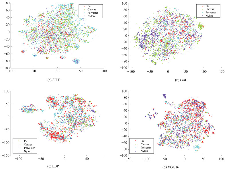
图 1 基于t-SNE的MattrSet数据集样本可视化结果(均为调参后的最佳效果)
Fig. 1 Visualization results of MattrSet dataset based on t-SNE(the best results are obtained after parameters tuning)
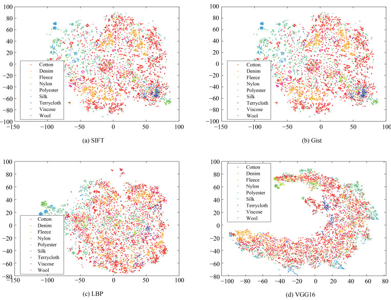
图 2 基于t-SNE的Fabric数据集样本可视化结果(均为调参后的最佳效果)
Fig. 2 Visualization results of Fabric dataset based on t-SNE(the best results are obtained after parameters tuning)
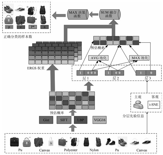
图 3 基于SGSMFF算法的材质属性标注模型(以MattrSet数据集为例, p表示Pu材质、p*表示Polyester材质、c表示Canvas材质、n表示Nylon材质. "1"表示正例, "0"表示负例)
Fig. 3 The proposed material attribute annotation model based on the SGSMFF algorithm(MattrSet is used as example, p, p*, c, n, "1", and "0" represent Pu, Polyester, Canvas, Nylon, positive, and negative examples, respectively )
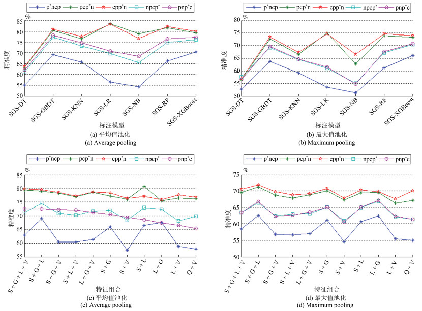
图 4 面向不同的SGS模型或不同特征组合的精准度均值比较
(a)和(b)是不同模型, (c)和(d)是不同特征组合
Fig. 4 The mean accuracy comparisons of different SGS models or feature combinations
(a) and (b) are different models, (c) and (d) are different feature combinations
表 1 各类材质的t-SNE代价值(针对不同数据集, 每列最小值如1.3079等所示)
Table 1 The t-SNE cost value of different material (for different dataset, the minimum value of each column is shown as 1.3079 etc.)
数据集 材质 t-SNE代价值 Gist SIFT LBP VGG 代价均值 MattrSet Pu 1.3079 1.4615 0.7735 0.9142 1.1143 Canvas 1.4517 1.7962 0.8653 0.9660 1.2698 Nylon 1.4077 1.7227 0.8333 0.9360 1.2249 Polyester 1.3948 1.7285 0.8318 0.9982 1.2383 Fabrc Cotton 1.0282 1.2109 1.2102 0.8974 1.0867 Denim 0.4405 0.9569 0.5581 0.4354 0.5977 Fleece 0.2267 0.5844 0.1583 0.1219 0.2728 Nylon 0.2219 0.1730 0.2105 0.1480 0.1884 Polyester 0.7151 0.9591 0.7243 0.5471 0.7364 Silk 0.1852 0.3642 0.1944 0.2078 0.2379 Terrycloth 0.2441 0.4616 0.3116 0.1457 0.2907 Viscose 0.2319 0.5017 0.2818 0.1035 0.2797 Wool 0.4072 0.6868 0.4417 0.2565 0.4480  下载: 导出CSV
表 2 SGS算法中的参数设置
Table 2 parameter settings of the proposed SGS algorithm
参数 $ T $ $CM $ ${y_i}$ $F$ $C $ D ${x_i}$ l N n k d cc cm \ 意义 图像数据集合 分类模型集合 图像样本标签 图像特征集合 材质属性标签集合 特征组合集合 图像样本 材质属性标签数 样本总数 特征总数 特征$fea{t_z}$的维度 特征组合总数 组合中的特征数 分类模型数量 \ 参数值 $\left\{ \begin{array}{*{35}{l}} \begin{align} & \left( {{x}_{1}},{{y}_{1}} \right),\cdots , \\ & \left( {{x}_{N}},{{y}_{N}} \right) \\ \end{align} \\ \end{array} \right\}$ $\left\{ \begin{array}{*{35}{l}} \begin{align} & Classifie{{r}_{1}},\cdots , \\ & Classifie{{r}_{cm}} \\ \end{align} \\ \end{array} \right\}$ ${y_i} \subseteq C$ $\begin{align} & \left\{ fea{{t}_{1}},fea{{t}_{2}},\cdots ,fea{{t}_{n}} \right\} \\ & fea{{t}_{z}}\subseteq {{\bf{R}}^{k}},z\in \left\{ 1,\cdots ,n \right\} \\ \end{align}$ $C =\left\{ {{c_1}, {c_2}, \cdots, {c_l}} \right\}$ $\begin{align} & \left\{ feat\_com{{b}_{1}},\cdots ,feat\_com{{b}_{d}} \right\} \\ & feat\_com{{b}_{i}}=\left\{ fea{{t}_{1}},\cdots ,fea{{t}_{cc}} \right\} \\ \end{align}$ \ MattrSet:4
Fabric:9MattrSet:11021
Fabric: 50644 Gist: 512
LBP: 1180
SIFT: 800
VGG16: 100011 单类别的特征: 1
两种特征融合: 2
两种特征融合: 3
两种特征融合: 47 \
下载: 导出CSV
表 4 MattrSet数据集上, GS类模型精准度及相对基本模型的Accuracy变化(每列最优值如46.20等表示, 单位: %)
Table 4 The accuracies of GS models and the corresponding accuracy variations compared to the basic models in the MattrSet dataset (The optimal value of each column is expressed as 46.20, etc., unit: %)
特征 GS类模型的Accuracy GS-DT GS-GBDT GS-KNN GS-LR GS-NB GS-RF GS-XGBoost S + G + L + V 42.33 59.83 54.89 54.57 49.12 59.14 61.23 S + G + L 46.20 65.13 62.10 58.41 44.87 61.70 67.67 S + G + V 42.40 57.67 51.52 50.72 49.25 57.47 59.27 S + L + V 42.35 57.45 51.33 53.04 39.23 57.29 58.94 L + G + V 42.42 59.09 54.37 52.59 41.66 58.98 59.87 S + G 45.31 62.48 58.32 53.22 49.61 60.14 64.39 S + V 42.49 53.98 41.76 46.36 47.85 55.13 56.54 S + L 37.12 62.95 57.56 59.45 46.05 58.92 63.75 L + G 45.65 63.79 60.90 57.34 40.88 61.75 65.08 L + V 42.26 56.20 50.19 50.43 40.37 56.40 57.52 G + V 42.28 56.40 50.10 47.00 43.49 56.69 57.63 $\Delta \rm{Accuracy}_\rm{M1}$ 1.45 2.99 3.52 5.25 3.01 3.36 2.97 $\Delta \rm{Accuracy}_\rm{M2}$ 0.96 3.85 5.77 3.61 1.25 1.99 4.74
下载: 导出CSV
表 3 基本分类模型的标注精准度(各数据集每列最优值如45.24等表示, 单位: %
Table 3 The accuracy of basic model (for each dataset, the optimal value of each column is expressed as 45.24, etc, unit: %)
数据集 特征 基本分类模型的Accuracy DT GBDT KNN LR NB RF XGBoost MattrSet L 43.67 61.28 56.33 55.84 40.86 59.76 62.93 S 34.40 52.41 43.73 50.48 48.36 47.96 52.90 G 45.24 60.34 56.05 49.19 43.27 59.32 61.99 V 42.11 52.17 45.45 35.52 34.51 53.55 54.64 Fabric L 47.31 70.02 68.17 69.15 27.17 62.40 70.38 S 67.10 79.66 37.84 80.85 56.60 75.79 82.03 G 51.90 70.70 71.37 55.63 51.80 68.33 73.42 V 49.45 65.01 57.46 58.10 46.88 64.34 66.59
下载: 导出CSV
表 5 Fabric数据集上, GS类模型精准度及其相对基本模型的Accuracy变化(每列最优值如79.98等表示, 单位: %)
Table 5 The accuracies of GS models and the corresponding accuracy variations compared to the basic models in the Fabric dataset (The optimal value of each column is expressed as 79.98, etc., unit: %)
特征 GS类模型的Accuracy GS-DT GS-GBDT GS-KNN GS-LR GS-NB GS-RF GS-XGBoost S + G + L + V 58.93 73.46 68.84 68.29 45.06 69.19 78.75 S + G + L 65.64 75.25 62.56 74.12 39.69 69.67 80.57 S + G + V 49.45 71.96 66.90 66.00 48.82 70.85 72.71 S + L + V 47.95 72.12 67.58 69.08 43.84 68.48 72.71 L + G + V 47.43 72.43 71.09 65.17 42.54 68.17 72.24 S + G 60.35 79.98 57.66 77.76 57.42 76.58 81.95 S + V 49.45 69.91 59.28 66.94 48.54 70.02 70.62 S + L 64.69 76.26 41.00 78.28 31.87 71.17 81.71 L + G 48.74 71.64 73.74 66.71 27.29 66.00 73.54 L + V 47.47 69.31 66.63 65.44 42.54 64.34 70.38 G + V 49.45 67.73 63.78 59.64 47.47 67.58 69.04 $\Delta \rm{Accuracy}_\rm{F1}$ -0.34 1.38 4.84 2.92 -2.42 1.56 1.82 $\Delta \rm{Accuracy}_\rm{F2}$ -1.46 0.32 2.37 -2.57 0.82 0.79 -0.08
下载: 导出CSV
表 6 MattrSet数据集中SGS_MAX类模型相对GS类模型的Accuracy变化值$ \Delta {\rm{Accurac}}{{\rm{y}}_{{\rm{M3}}}}$ (性能衰减如-0.20所示, 单位: %)
Table 6 The accuracy variations of the SGS_MAX model compared to the GS model in the MattrSet dataset: $\Delta {\rm{Accurac}}{{\rm{y}}_{{\rm{M3}}}}$ (The performance degradation indicators are marked in -0.20, unit: %)
${\rm{SP}}{{\rm{I}}_{\rm{M}}}$ SGS模型 $\Delta \text{Accurac}{{\text{y}}_{\text{M3}}}\text{=Accurac}{{\text{y}}_{\text{SGS }\!\!\_\!\!\text{ }}}_{\text{MAX}}\text{-Accurac}{{\text{y}}_{\text{GS}}} $ all S + G + L S + G + V S + L + V L + G +V S + G S + V S + L L + G L + V G + V ${\rm{Av}}{{\rm{g}}_{{\rm{model}}}}$ pcp*n
SPIM-1
SPIM-3
SPIM-4DT 14.27 10.02 14.11 14.19 14.21 12.98 14.00 14.56 13.58 14.85 14.68 13.77 GBDT 12.81 12.51 13.29 13.71 12.30 13.23 14.69 13.92 11.29 13.27 13.29 13.12 KNN 12.45 8.93 13.01 13.16 12.34 10.60 20.50 10.46 9.84 13.83 14.23 12.67 LR 22.96 17.03 24.25 24.29 23.83 20.06 27.81 16.04 14.89 25.06 26.72 22.09 NB 16.21 16.61 20.44 22.00 23.92 11.49 21.65 12.18 16.17 16.83 20.53 18.00 RF 14.81 16.84 14.94 15.17 13.83 16.77 15.08 19.21 14.89 14.16 14.34 15.46 XGBoost 12.00 10.15 12.47 12.76 12.34 11.34 12.95 13.83 10.87 12.89 12.89 12.23 pnp*c
SPIM-2
SPIM-5DT 14.89 10.05 14.03 14.28 15.63 11.32 12.09 15.30 13.98 15.16 14.57 13.75 GBDT 9.71 7.75 10.76 11.00 10.00 9.20 12.40 8.22 9.18 11.45 11.53 10.11 KNN 9.62 6.15 11.34 11.35 10.40 8.41 18.47 8.13 9.19 12.02 12.54 10.69 LR 5.75 7.54 8.29 7.03 7.06 8.86 11.11 9.33 9.73 7.95 10.89 8.50 NB 6.15 15.10 3.65 15.43 13.87 7.41 3.85 12.98 13.43 14.09 4.47 10.04 RF 8.22 8.04 9.33 9.35 9.02 8.09 10.87 7.01 9.28 10.76 10.44 9.13 XGBoost 9.00 6.48 10.31 10.33 10.54 8.64 10.79 8.46 9.62 11.28 11.40 9.71 p*ncp
SPIM-6DT 10.98 7.08 10.71 10.58 10.62 8.95 8.64 11.06 9.99 10.20 10.05 9.90 GBDT 3.97 3.03 4.08 4.41 4.64 3.18 4.78 2.38 5.10 5.52 5.30 4.22 KNN 3.31 2.83 4.48 5.18 4.13 5.27 10.92 5.46 5.10 6.23 5.54 5.31 LR ${\bf{-0.20}}$ 0.89 0.00 0.33 ${\bf{-0.40}}$ 0.71 0.00 1.83 2.43 ${\bf{-0.20}} $ 0.01 0.49 NB 3.59 13.89 2.14 8.17 2.43 10.76 4.12 13.74 10.62 2.65 0.00 6.56 RF 2.27 1.51 2.81 2.78 3.34 1.43 3.57 0.85 3.27 4.32 4.21 2.76 XGBoost 4.66 2.69 4.81 5.45 5.77 3.63 6.08 3.12 5.24 6.58 6.39 4.95 p*pcn
SPIM-7DT 15.50 9.71 15.31 15.65 15.05 13.76 14.73 15.88 14.85 15.90 15.92 14.75 GBDT 8.79 7.08 9.22 9.99 9.76 7.75 16.25 8.19 8.82 11.20 10.60 9.79 KNN 8.68 5.50 10.18 10.22 9.73 8.28 17.25 6.83 8.11 12.05 12.09 9.90 LR 6.42 7.79 8.47 7.35 7.77 9.48 11.15 8.15 9.79 8.67 11.10 8.74 NB 10.76 17.81 6.39 17.91 13.36 11.22 8.39 14.47 17.15 15.70 4.50 12.51 RF 7.79 6.30 8.49 9.09 8.62 6.61 9.78 6.57 7.57 10.24 9.66 8.25 XGBoost 9.02 6.55 9.60 10.22 9.92 7.49 10.57 7.99 8.25 11.19 10.91 9.25 cpp*n
SPIM-8DT 14.32 11.16 14.25 14.52 14.29 13.34 14.27 15.09 13.11 14.23 15.10 13.97 GBDT 13.89 12.09 15.30 15.07 13.72 13.61 16.07 13.82 11.00 14.38 15.05 14.00 KNN 13.31 9.96 14.19 14.69 13.48 10.42 19.92 11.69 10.35 14.40 15.70 13.46 LR 22.94 17.77 23.78 23.36 22.81 21.22 26.76 16.41 15.60 23.61 24.94 21.75 NB 18.71 19.44 22.45 24.18 22.96 15.25 23.32 15.78 16.99 24.22 35.93 21.75 RF 16.08 16.44 16.45 16.43 15.21 16.33 16.72 19.10 15.00 15.61 15.86 16.29 XGBoost 12.89 9.60 13.77 13.72 13.03 11.76 13.89 13.81 10.87 13.55 13.89 12.80 npcp*
SPIM-9DT 15.30 12.20 14.67 14.70 14.90 13.25 13.94 19.79 14.12 14.86 14.99 14.79 GBDT 9.33 6.75 10.47 10.89 9.80 8.60 12.33 7.24 8.82 11.02 11.38 9.69 KNN 9.71 6.13 11.40 11.33 10.25 8.17 18.31 8.84 8.80 11.71 12.82 10.68 LR 6.06 6.57 8.31 7.32 4.08 8.61 11.15 8.04 8.75 8.40 10.98 8.02 NB 6.59 14.25 4.19 17.84 15.01 7.81 4.86 10.22 14.05 14.10 4.58 10.32 RF 7.90 6.64 9.31 9.27 8.64 7.59 10.60 6.85 9.03 10.22 10.18 8.75 XGBoost 8.71 5.83 10.31 10.40 10.22 8.09 11.00 7.66 9.16 11.04 11.15 9.42 $\rm{Avg}_\rm{Feat}$ 10.48 9.54 11.09 12.26 11.49 10.02 12.99 10.73 10.66 12.27 12.18 /
下载: 导出CSV
表 7 Fabric数据集中SGS_MAX类模型相对GS类模型的Accuracy变化值$ \Delta \rm{Accuracy}_\rm{F3}$ (性能衰减如$ \bf{{-3.47}}$所示, 单位: %)
Table 7 The accuracy variations of the SGS_MAX model compared to the GS model in the Fabric dataset: $\Delta \rm{Accuracy}_\rm{F3}$ (The performance degradation indicators are marked in ${\bf{-3.47}}$, unit: %)
$\text{SP}{{\text{I}}_{\text{F}}}$ SGS模型 $\Delta \text{Accurac}{{\text{y}}_{\text{F3}}}\text{=Accurac}{{\text{y}}_{\text{SGS }\!\!\_\!\!\text{ MAX}}}\text{-}\text{Accurac}{{\text{y}}_{\text{GS}}}$ all S + G + L S + G + V S + L + V L + G + V S + G S + V S + L L + G L + V G + V $\text{Av}{{\text{g}}_{\text{model}}}$ SPIF-1 DT 8.01 6.32 16.62 18.40 13.00 5.80 36.41 9.24 39.14 11.22 10.86 15.91 GBDT 15.36 15.31 16.35 15.99 13.98 11.25 16.78 14.02 15.80 15.92 17.06 15.26 KNN 6.79 0.59 8.34 0.63 13.82 1.98 6.30 3.19 12.08 12.36 17.97 7.64 LR 18.87 15.97 20.18 19.07 18.36 11.73 20.54 12.79 15.83 18.37 20.85 17.51 NB 33.47 24.49 29.70 30.65 27.92 15.41 28.71 35.55 23.46 27.68 27.57 27.69 RF 18.33 18.72 16.55 17.74 16.86 12.99 15.45 16.55 19.19 18.60 16.82 17.07 XGBoost 11.26 11.25 16.86 15.88 15.48 10.27 15.24 10.00 15.64 15.32 17.18 14.03 SPIF-2 DT 7.74 5.57 15.56 18.24 15.88 8.05 17.18 9.36 12.16 14.10 12.24 12.37 GBDT 0.87 3.23 1.70 1.73 ${\bf{ -1.18}} $ 1.10 4.46 4.86 1.31 0.91 2.77 1.98 KNN 6.24 19.00 5.61 3.63 2.33 22.55 9.91 39.45 5.64 2.37 7.19 11.27 LR 0.94 4.12 0.82 2.05 ${\bf{-0.52}} $ 2.02 4.78 4.42 1.73 1.28 1.77 2.13 NB 6.32 29.15 1.02 6.75 6.43 19.99 3.79 45.58 32.86 6.59 1.27 14.52 RF ${\bf{-17.81}}$ 5.09 0.79 2.22 0.43 1.38 2.61 4.15 1.65 2.96 1.38 0.44 XGBoost $ {\bf{-3.47}} $ ${\bf{-0.16}} $ 2.09 1.30 0.75 1.42 4.22 0.83 1.66 1.22 3.31 1.20 $ \rm{Avg}_\rm{Feat}$ 8.07 11.33 10.87 11.02 10.25 9.00 13.31 15.00 14.15 10.64 11.30 /
下载: 导出CSV
表 8 MattrSet数据集中, SGS_AVG类模型相对SGS_MAX类模型Accuracy变化值$ \Delta \rm{Accuracy}_\rm{M4}$ (性能衰减用${\bf{-3.82}}$表示, 单位: %)
Table 8 The accuracy variations of the SGS_AVG model compared to the SGS_MAX model in the MattrSet dataset: $ \Delta \rm{Accuracy}_\rm{M4}$ (The performance degradation indicators are marked in ${\bf{-3.82}}$, unit: %)
SPIM} SGS模型 $\Delta \rm{Accuracy}_\rm{M4}=\rm{Accuracy}_\rm{SGS_AVG}\, -\, \rm{Accuracy}_\rm{SGS_MAX}$ all S + G + L S + G + V S + L + V L + G + V S + G S + V S + L L + G L + V G + V $\rm{Avg}_\rm{model}$ SPIM-1 DT 7.75 14.72 5.32 3.56 6.88 9.54 0.18 15.28 10.11 0.14 0.13 6.69 GBDT 8.39 5.62 9.13 8.95 8.28 6.26 8.80 6.58 5.19 8.77 8.60 7.69 KNN 10.95 9.17 11.13 11.59 10.76 8.28 9.11 9.62 7.66 10.40 10.11 9.89 LR 7.91 6.95 8.91 8.17 8.33 7.30 10.65 6.54 7.08 9.73 9.53 8.28 NB 18.30 6.72 16.61 15.26 18.94 7.28 16.87 7.48 0.37 27.23 20.48 14.14 RF 8.50 5.78 8.60 8.95 7.93 6.28 9.22 6.31 6.02 8.73 8.31 7.69 XGBoost 7.04 4.75 6.80 6.74 6.35 5.56 6.11 5.81 4.16 5.77 5.94 5.91 SPIM-8 DT 8.92 11.26 4.00 3.49 5.06 9.57 0.20 14.83 10.44 7.12 0.22 6.83 GBDT 7.37 7.26 7.14 7.78 7.15 6.65 7.73 6.97 6.15 9.51 7.17 7.35 KNN 11.32 9.77 11.13 10.53 10.26 9.51 10.67 9.69 7.98 11.78 9.04 10.15 LR 8.30 6.68 9.78 9.42 9.72 6.65 12.01 6.70 6.69 5.59 12.16 8.52 NB 15.11 6.36 14.60 13.03 19.90 7.84 15.20 ${\bf{-3.82}} $ 0.14 19.25 5.08 10.24 RF 7.55 6.78 7.35 7.71 7.13 7.21 7.77 6.80 6.50 8.29 7.30 7.31 XGBoost 6.62 5.76 6.07 6.54 6.37 5.30 5.65 6.16 4.68 7.87 5.61 6.06 $\rm{Avg}_\rm{Feat}$ 9.57 7.68 9.04 8.69 9.50 7.37 8.58 7.50 5.94 10.01 7.83 /
下载: 导出CSV
表 9 Fabric数据集中, SGS_AVG类模型相对SGS_MAX类模型的Accuracy变化值$\Delta \rm{Accuracy}_\rm{F4}$ (性能衰减用${\bf{ -16.36}}$表示, 单位: %)
Table 9 The accuracy variations of the SGS_AVG model compared to the SGS_MAX model in the Fabric dataset: $\Delta \text{Accurac}{{\text{y}}_{\text{F4}}}$ (The performance degradation indicators are marked in ${\bf{ -16.36}}$, unit: %)
SPIF SGS模型 $\Delta \rm{Accuracy}_\rm{F4}=\rm{Accuracy}_\rm{SGS_AVG}\, -\, \rm{Accuracy}_\rm{SGS_MAX}$ all S + G + L S + G + V S + L + V L + G + V S + G S + V S + L L + G L + V G + V $\rm{Avg}_\rm{model}$ SPIF-1 DT 20.94 14.41 17.74 19.12 19.90 15.88 $ {\bf{ -4.58}}$ 6.56 -16.36 10.86 12.75 10.66 GBDT 7.19 5.14 7.42 7.39 8.42 4.27 8.29 4.63 6.08 8.45 8.73 6.91 KNN 19.31 29.86 18.99 24.29 11.06 30.25 24.03 40.25 9.28 14.89 13.06 21.39 LR 10.31 7.46 11.06 9.32 10.98 6.93 9.36 6.17 11.93 10.54 12.32 9.67 NB 15.94 25.04 16.39 18.64 13.11 17.85 16.31 6.55 24.37 10.31 6.00 15.50 RF 9.48 8.41 9.64 10.58 11.65 7.39 11.22 8.49 10.66 13.03 11.89 10.22 XGBoost 7.34 5.10 7.71 8.49 8.49 4.42 10.63 4.66 6.08 9.24 8.53 7.34 SPIF-2 DT 8.88 8.21 5.61 4.98 4.03 4.19 2.25 4.07 4.82 2.17 2.84 4.73 GBDT 7.98 8.01 7.62 7.90 5.61 5.69 5.25 5.97 5.76 4.74 5.33 6.35 KNN 10.23 7.46 10.47 11.02 9.08 7.51 6.21 6.24 7.35 9.48 9.32 8.58 LR 12.56 11.73 12.01 12.84 8.02 7.98 8.61 9.01 9.29 7.29 7.03 9.67 NB 13.15 10.27 12.80 13.80 8.65 0.91 10.51 3.47 0.24 10.23 3.12 7.92 RF 29.74 8.38 9.72 10.64 8.93 6.60 7.31 8.25 8.85 8.81 8.57 10.53 XGBoost 9.08 8.93 8.61 8.85 6.59 6.44 6.12 6.99 6.67 5.41 5.89 7.23 AvgFeat 13.01 11.32 11.13 11.99 9.61 9.02 8.68 8.67 6.79 8.96 8.24 /
下载: 导出CSV
表 10 MattrSet数据集中, 各基线最优值与本文模型的Accuracy比较(最优值如86.37等表示, 单位: %)
Table 10 The best accuracy of each baseline in the MattrSet dataset is compared with the proposed model (The best value is marked as 86.37, etc., unit: %)
Model Accuracy Model Accuracy 1) SVM-S 50.83 2) GS-DT-SGL 46.20 3) GBDT-L 61.28 4) GS-RF-LG 61.75 5) Adaboost-L 61.54 6) GS-KNN-SGL 62.10 7) XGBoost-L 62.93 8) GS-LR-SL 59.45 9) VGG16 33.98 10) GS-NB-SG 49.61 11) InceptionResNetV2 52.09 12) GS-GBDT-SGL 65.13 13) Densenet169 59.77 14) GS-Adaboost-SGL 66.11 15) MobileNets 33.98 16) GS-XGBoost-SGL[64] 67.67 17) p*ncp-a-SGS-XGBoost-SGL 75.71 18) p*ncp-m-SGS-XGBoost-SGL 70.36 19) cpp*n-a-SGS-NB-SV 86.37 20) cpp*n-m-SGS-RF-SGL 78.14 21) p*pcn-a-SGS-XGBoost-SGL 80.00 22) p*pcn-m-SGS-XGBoost-SGL 74.22 23) pcp*n-a-SGS-NB-SV 86.37 24) pcp*n-m-SGS-RF-SGL 78.54 25) pnp*c-a-SGS-GBDT-SGL 80.05 26) pnp*c-m-SGS-XGBoost-LG 74.70 27) npcp*-a-SGS-GBDT-SGL 79.71 28) npcp*-m-SGS-XGBoost-LG 74.24
下载: 导出CSV
表 11 Fabric数据集中, 各基线最优值与本文模型的Accuracy比较(最优值如97.55等表示, 单位: %)
Table 11 The best accuracy of each baseline in the Fabric dataset is compared with the proposed model (The best value is marked as 97.55, etc., unit: %)
Model Accuracy Model Accuracy 1) SVM-S 77.92 2) GS-DT-SGL 65.64 3) GBDT-S 79.66 4) GS-RF-SG 76.58 5) AdaBoost-S 76.86 6) GS-KNN-LG 73.74 7) XGBoost-S 82.03 8) GS-LR-SL 78.28 9) VGG16 46.22 10) GS-NB-SG 57.42 11) VGG-M[35] 79.60 12) GS-GBDT-SG 79.98 13) Densenet169 46.22 14) GS-AdaBoost-SL 78.16 15) MobileNet 46.22 16) GS-XGBoost-SG[64] 81.95 17) sdtcvpfnw-m-SGS-XGBoost-SG 92.22 18) sdtcvpfnw-a-SGS-LR-SGL 97.55 19) nsfvtwdpc-m-SGS-XGBoost-SG 83.37 20) nsfvtwdpc-a-SGS-LR-SL 91.71
下载: 导出CSV
表 12 MattrSet数据集中材质属性与实用属性之间的映射关系
Table 12 The relationship between the material attributes and their utility attributes in the MattrSet dataset
材质属性 二元映射关系 相对映射关系 防水性 透气性 柔软性 水洗性 耐磨性 防水性 透气性 柔软性 水洗性 耐磨性 Pu (皮革) 1 0 0 0 0 4 2 1 1 1 Canvas (帆布) 0 1 0 1 1 1 4 2 4 4 Polyester (涤纶) 1 0 1 1 0 3 1 4 2 3 Nylon (尼龙) 0 0 1 1 0 2 3 3 3 2
下载: 导出CSV
表 13 Fabric数据集中材质属性与实用属性之间的映射关系
Table 13 The relationship between the material attributes and their utility attributes in the Fabric dataset
材质属性 二元映射关系 相对映射关系 防水性 透气性 柔软性 耐磨性 防水性 透气性 柔软性 耐磨性 Wool (羊毛) 0 1 1 0 1 8 8 1 Denim (牛仔布) 0 0 0 1 8 1 1 8 Viscose (粘胶纤维) 0 1 1 1 7 7 6 9 Cotton (棉花) 0 1 1 0 4 5 5 3 Silk (丝绸) 0 1 1 0 5 9 9 5 Polyester (涤纶) 1 0 1 0 9 2 3 7 Nylon (尼龙) 0 0 1 0 6 3 2 6 Terrycloth (毛巾布) 0 1 1 1 3 4 4 4 Fleece (摇粒绒) 0 1 1 0 2 6 7 2
下载: 导出CSV
-
[1] Krishna R, Zhu Y K, Groth O, Johnson J, Hata K, Kravitz J, et al. Visual genome: Connecting language and vision using crowdsourced dense image annotations. International Journal of Computer Vision, 2017, 123(1): 32-73 http://dl.acm.org/citation.cfm?id=3089101 [2] Pietikäinen M, Hadid A, Zhao G Y, Ahonen T. Computer Vision Using Local Binary Patterns. London: Springer Berlin, 2011. [3] Oliva A, Torralba A. Building the gist of a scene: The role of global image features in recognition. Progress in Brain Research, 2006, 155: 23-36 doi: 10.1016/S0079-6123(06)55002-2 [4] Lowe D G. Distinctive image features from scale-invariant keypoints. International Journal of Computer Vision, 2004, 60(2): 91-110 http://dl.acm.org/citation.cfm?id=996342&CFID=520673225&CFTOKEN=77943935 [5] Simonyan K, Zisserman A. Very deep convolutional networks for large-scale image recognition. In: Proceedings of the 3rd International Conference on Learning Representations. San Diego, CA, USA, 2015. 1-14 [6] Chandra B, Gupta M. An efficient statistical feature selection approach for classification of gene expression data. Journal of Biomedical Informatics, 2011, 44(4): 529-535 http://dl.acm.org/citation.cfm?id=2010675 [7] Farhadi A, Endres I, Hoiem D, David F. Describing objects by their attributes. In: Proceedings of the 2009 IEEE Conference on Computer Vision and Pattern Recognition, 2009: 1778-1785 doi: 10.1109/CVPRW.2009.5206772 [8] Kumar N, Belhumeur P, Nayar S. FaceTracer: A search engine for large collections of images with faces. In: Proceedings of the 10th European Conference on Computer Vision. Marseille, France: Springer, 2008. 340-353 [9] Kumar N, Berg A C, Belhumeur P N, Nayar S K. Attribute and simile classifiers for face verification. In: Proceedings of the 12th International Conference on Computer Vision. Kyoto, Japan: IEEE, 2009. 365-372 [10] Jayaraman D, Grauman K. Zero-shot recognition with unreliable attributes. In: Proceedings of the 27th International Conference on Neural Information Processing Systems. Montreal, Quebec, Canada: MIT Press, 2014. 3464-3472 [11] Berg T L, Berg A C, Shih J. Automatic attribute discovery and characterization from noisy web data. In: Proceedings of the 11th European Conference on Computer Vision. Heraklion, Greece: Springer, 2010. 663-676 [12] Gan C, Yang T B, Gong B Q. Learning attributes equals multi-source domain generalization. In: Proceedings of the 2016 IEEE Conference on Computer Vision and Pattern Recognition. Las Vegas, USA: IEEE, 2016. 87-97 [13] Liu Z W, Luo P, Wang X G, Tang X O. Deep learning face attributes in the wild. In: Proceedings of the 2015 IEEE International Conference on Computer Vision. Santiago, Chile: IEEE, 2015. 3730-3738 [14] Tang P, Zhang J, Wang X G, Feng B, Roli F B, Liu W Y. Learning extremely shared middle-level image representation for scene classification. Knowledge and Information Systems, 2017, 52(2): 509-530 http://www.wanfangdata.com.cn/details/detail.do?_type=perio&id=414a554cd565e9f2c284abfe28edbdd1 [15] Bradley C, Boult T E, Ventura J. Cross-modal facial attribute recognition with geometric features. In: Proceedings of the 12th IEEE International Conference on Automatic Face & Gesture Recognition. Washington, USA: IEEE, 2017. 891-896 [16] Liu Z W, Luo P, Qiu S, Wang X G, Tang X O. DeepFashion: Powering robust clothes recognition and retrieval with rich annotations. In: Proceedings of the 2016 IEEE Conference on Computer Vision and Pattern Recognition. Las Vegas, USA: IEEE, 2016. 1096-1104 [17] Qi G J, Hua X S, Rui Y, Tang J H, Mei T, Zhang H J. Correlative multi-label video annotation. In: Proceedings of the 15th ACM International Conference on Multimedia. Augsburg, Germany: ACM, 2007. 17-26 [18] Parikh D, Grauman K. Relative attributes. In: Proceedings of the 2011 International Conference on Computer Vision. Barcelona, Spain: IEEE, 2011. 503-510 [19] Kovashka A, Grauman K. Attribute adaptation for personalized image search. In: Proceedings of the 2013 IEEE International Conference on Computer Vision. Sydney, Australia: IEEE, 2013. 3432-3439 [20] Kovashka A, Parikh D, Grauman K. WhittleSearch: Interactive image search with relative attribute feedback. International Journal of Computer Vision, 2015, 115(2): 185-210 http://d.wanfangdata.com.cn/periodical/613be5470b6e7be562fc6e807806b4d8 [21] Yu A, Grauman K. Just noticeable differences in visual attributes. In: Proceedings of the 2015 International Conference on Computer Vision. Santiago, Chile: IEEE, 2015. 2416-2424 [22] Cheng Y H, Qiao X, Wang X S, Yu Q. Random forest classifier for zero-shot learning based on relative attribute. IEEE Transactions on Neural Networks and Learning Systems, 2018, 29(5): 1662-1674 doi: 10.1109/TNNLS.2017.2677441 [23] Yuan B D, Tu J, Zhao R W, ZhengY B, Jiang Y G. Learning part-based mid-level representation for visual recognition. Neurocomputing, 2018, 275: 2126-2136 doi: 10.1016/j.neucom.2017.10.062 [24] Liu X, Wang J, Wen S L, Ding E R, Lin Y Q. Localizing by describing: Attribute-guided attention localization for fine-grained recognition. In: Proceedings of the 31st AAAI Conference on Artificial Intelligence. San Francisco, California, USA: AAAI, 2017. 4190-4196 [25] Ledig C, Theis L, Huszar F, Caballero J, Cunningham A, Acosta A, et al. Photo-realistic single image super-resolution using a generative adversarial network[Online], available: https://arxiv.org/abs/1609.04802, September 15, 2016. [26] Singh K K, Lee Y J. End-to-end localization and ranking for relative attributes. In: Proceedings of the 14th European Conference on Computer Vision. Amsterdam, The Netherlands: Springer, 2016. 753-769 [27] Liu X G, Yu Y Z, Shum H Y. Synthesizing bidirectional texture functions for real-world surfaces. In: Proceedings of the 28th Annual Conference on Computer Graphics and Interactive Techniques. New York, USA: ACM, 2001. 97-106 [28] Leung T, Malik J. Representing and recognizing the visual appearance of materials using three-dimensional textons. International Journal of Computer Vision, 2001, 43(1): 29-44 http://www.wanfangdata.com.cn/details/detail.do?_type=perio&id=d84bc2da159ff99e8d8f4c67b6af5546 [29] Varma M, Zisserman A. A statistical approach to texture classification from single images. International Journal of Computer Vision, 2005, 62(1-2): 61-81 doi: 10.1007/s11263-005-4635-4 [30] Heera M M, Divya J K, Varma M S, Divya R A, Agrawal D V K. Minimum variance optimal filter design for a 3x3 MEMS gyroscope cluster configuration. IFAC-Papersonline, 2016, 49(1): 639-645 doi: 10.1016/j.ifacol.2016.03.128 [31] Sharan L, Rosenholtz R, Adelson E. Material perception: What can you see in a brief glance? Journal of Vision, 2009, 9(8): 784 [32] Liu C, Sharan L, Adelson E H, Rosenholtz R. Exploring features in a Bayesian framework for material recognition. In: Proceedings of the 2010 IEEE Computer Society Conference on Computer Vision and Pattern Recognition. San Francisco, USA: IEEE, 2010. 239-246 [33] Hu D E, Bo L F, Ren X F. Toward robust material recognition for everyday objects. In: Proceedings of the 2011 British Machine Vision Conference. Dundee, UK: BMVA Press, 2011. 1-11 [34] Sharan L, Liu C, Rosenholtz R, Adelson E H. Recognizing materials using perceptually inspired features. International Journal of Computer Vision, 2013, 103(3): 348-371 doi: 10.1007/s11263-013-0609-0 [35] Kampouris C, Zafeiriou S, Ghosh A, Malassiotis S. Fine-grained material classification using micro-geometry and reflectance. In: Proceedings of the 14th European Conference on Computer Vision. Amsterdam, The Netherlands: Springer, 2016. 778-792 [36] Dong J Y, Chantler M. Capture and synthesis of 3D surface texture. International Journal of Computer Vision, 2005, 62(1-2): 177-194 doi: 10.1007/s11263-005-4641-6 [37] Jian M W, Yin Y L, Dong J Y, Zhang W Y. Comprehensive assessment of non-uniform illumination for 3D heightmap reconstruction in outdoor environments. Computers in Industry, 2018, 99: 110-118 doi: 10.1016/j.compind.2018.03.034 [38] Jian M W, Dong J Y. Capture and fusion of 3d surface texture. Multimedia Tools and Applications, 2011, 53(1): 237-251 doi: 10.1007/s11042-010-0509-z [39] Jian M W, Lam K M, Dong J Y. Illumination-insensitive texture discrimination based on illumination compensation and enhancement. Information Sciences, 2014, 269: 60-72 doi: 10.1016/j.ins.2014.01.019 [40] Van Der Maaten L, Hinton G. Visualizing data using t-SNE. Journal of Machine Learning Research, 2008, 9(11): 2579-2605 http://www.mendeley.com/catalog/visualizing-data-using-tsne/ [41] Friedman J H. Greedy function approximation: A gradient boosting machine. The Annals of Statistics, 2001, 29(5): 1189-1232 http://bioscience.oxfordjournals.org/external-ref?access_num=10.1214/aos/1013203451&link_type=DOI [42] 侯杰, 茅耀斌, 孙金生.基于指数损失和0-1损失的在线Boosting算法.自动化学报, 2014, 40(4): 635-642 doi: 10.3724/SP.J.1004.2014.00635Hou Jie, Mao Yao-Bin, Sun Jin-Sheng. Online boosting algorithms based on exponential and 0-1 loss. Acta Automatica Sinica, 2014, 40(4): 635-642 doi: 10.3724/SP.J.1004.2014.00635 [43] Vu H T, Gallinari P. Using RankBoost to compare retrieval systems. In: Proceedings of the 14th ACM International Conference on Information and Knowledge Management. Bremen, Germany: ACM, 2005. 309-310 [44] Chen T Q, Guestrin C. XGBoost: A scalable tree boosting system. In: Proceedings of the 22nd ACM SIGKDD International Conference on Knowledge Discovery and Data Mining. San Francisco, USA: ACM, 2016. 785-794 [45] Feng J, Yu Y, Zhou Z H. Multi-layered gradient boosting decision trees. In: Proceedings of the 32nd Conference on Neural Information Processing Systems. Montréal, Canada: 2018. [46] Vedaldi A, Gulshan V, Varma M, Zisserman A. Multiple kernels for object detection. In: Proceedings of the 2009 IEEE 12th International Conference on Computer Vision. Kyoto, Japan: IEEE, 2009. 606-613 [47] Xia H, Hoi S C H. MKBoost: A framework of multiple kernel boosting. IEEE Transactions on Knowledge and Data Engineer, 2013, 25(7): 1574-1586 doi: 10.1109/TKDE.2012.89 [48] Zhang Z Y, Lyons M, Schuster M, Akamatsu S. Comparison between geometry-based and gabor-wavelets-based facial expression recognition using multi-layer perceptron. In: Proceedings of the 3rd IEEE International Conference on Automatic Face and Gesture Recognition. Nara, Japan: IEEE, 1998. 454-459 [49] Bai S, Sun S Y, Bai X, Zhang Z X, Tian Q. Smooth neighborhood structure mining on multiple affinity graphs with applications to context-sensitive similarity. In: Proceedings of the 14th European Conference on Computer Vision. Amsterdam, The Netherlands: Springer, 2016. 592-608 [50] 徐丹蕾, 杜兰, 刘宏伟, 洪灵, 李彦兵.一种基于变分相关向量机的特征选择和分类结合方法.自动化学报, 2011, 37(8): 932-943 doi: 10.3724/SP.J.1004.2011.00932Xu Dan-Lei, Du Lan, Liu Hong-Wei, Hong Ling, Li Yan-Bing. Joint feature selection and classification design based on variational relevance vector machine. Acta Automatica Sinica, 2011, 37(8): 932-943 doi: 10.3724/SP.J.1004.2011.00932 [51] Liu Z Q, Wang S J, Zheng L, Tian Q. Robust ImageGraph: Rank-level feature fusion for image search. IEEE Transactions on Image Processing, 2017, 26(7): 3128-3141 doi: 10.1109/TIP.2017.2660244 [52] Mafarja M, Aljarah I, Heidari A A, Hammouri A I, Faris H, Al-Zoubi A M, et al. Evolutionary population dynamics and grasshopper optimization approaches for feature selection problems. Knowledge-Based Systems, 2018, 145: 25-45 doi: 10.1016/j.knosys.2017.12.037 [53] Faris H, Mafarja M M, Heidari A A, Aljarah I, Al-Zoubi M, Mirjalili S, et al. An efficient binary salp swarm algorithm with crossover scheme for feature selection problems. Knowledge-Based System, 2018, 154: 43-67 doi: 10.1016/j.knosys.2018.05.009 [54] Emary E, Zawbaa H M, Grosan C, Hassenian A E. Feature subset selection approach by gray-wolf optimization. In: Proceedings of the 1st International Afro-European Conference for Industrial Advancement. Cham, Germany: Springer, 2014. 1-13 [55] Cox D R. The regression analysis of binary sequences. Journal of the Royal Statistical Society: Series B (Methodological), 1958, 20(2): 215-232 doi: 10.1111/j.2517-6161.1958.tb00292.x [56] Ho T K. Random decision forests. In: Proceedings of the 3rd International Conference on Document Analysis and Recognition. Montreal, Canada: IEEE, 1995. 278-282 https://ieeexplore.ieee.org/document/598994 [57] Altman N S. An introduction to kernel and nearest-neighbor nonparametric regression. The American Statistician, 1992, 46(3): 175-185 http://www.wanfangdata.com.cn/details/detail.do?_type=perio&id=10.1080/00031305.1992.10475879 [58] Quilan J R. Decision trees and multi-valued attributes. Machine Intelligence 11. New York, USA: Oxford University Press, 1988. 305-318 [59] Kononenko I. ID3, sequential Bayes, naive Bayes and Bayesian neural networks. In: Proceedings of European Working Session on Learning. 1989. 91-98 [60] Garreta R, Moncecchi G. Learning Scikit-Learn: Machine Learning in Python. Birmingham, England: Packt Publishing, 2013. [61] Szegedy C, Ioffe S, Vanhoucke V, Alemi A A. Inception-v4, inception-ResNet and the impact of residual connections on learning. In: Proceedings of the 31st AAAI Conference on Artificial Intelligence. San Francisco, California, USA: AAAI, 2017. 4278-4284 [62] Huang G, Liu Z, Van Der Maaten L, Weinberger K Q. Densely connected convolutional networks. In: Proceedings of the 2017 IEEE Conference on Computer Vision and Pattern Recognition. Honolulu, USA: IEEE, 2017. 2261-2269 https://ieeexplore.ieee.org/document/8099726 [63] Howard A G, Zhu M L, Chen B, Kalenichenko D, Wang W J, Weyand T, et al. MobileNets: Efficient convolutional neural networks for mobile vision applications[Online], available: https://arxiv.org/abs/1704.04861, April 17, 2017. [64] Zhang H B, Qiu D D, Wu Rv Z, Deng Y X, Ji D H, Li T. Novel framework for image attribute annotation with gene selection XGBoost algorithm and relative attribute model. Applied Soft Computing, 2019, 80: 57-79 doi: 10.1016/j.asoc.2019.03.017 [65] Chen W H, Chen X T, Zhang J G, Huang K Q. Beyond triplet loss: A deep quadruplet network for person re-identification. In: Proceedings of the 2017 IEEE Conference on Computer Vision and Pattern Recognition. Honolulu, USA: IEEE, 2017. 1320 -1329 [66] Odena A, Olah C, Shlens J. Conditional image synthesis with auxiliary classifier GANs. In: Proceedings of the 34th International Conference on Machine Learning. Sydney, Australia, 2017. -

 下载:
下载:

计量
- 文章访问数: 1313
- HTML全文浏览量: 251
- PDF下载量: 151
- 被引次数: 0
