

-
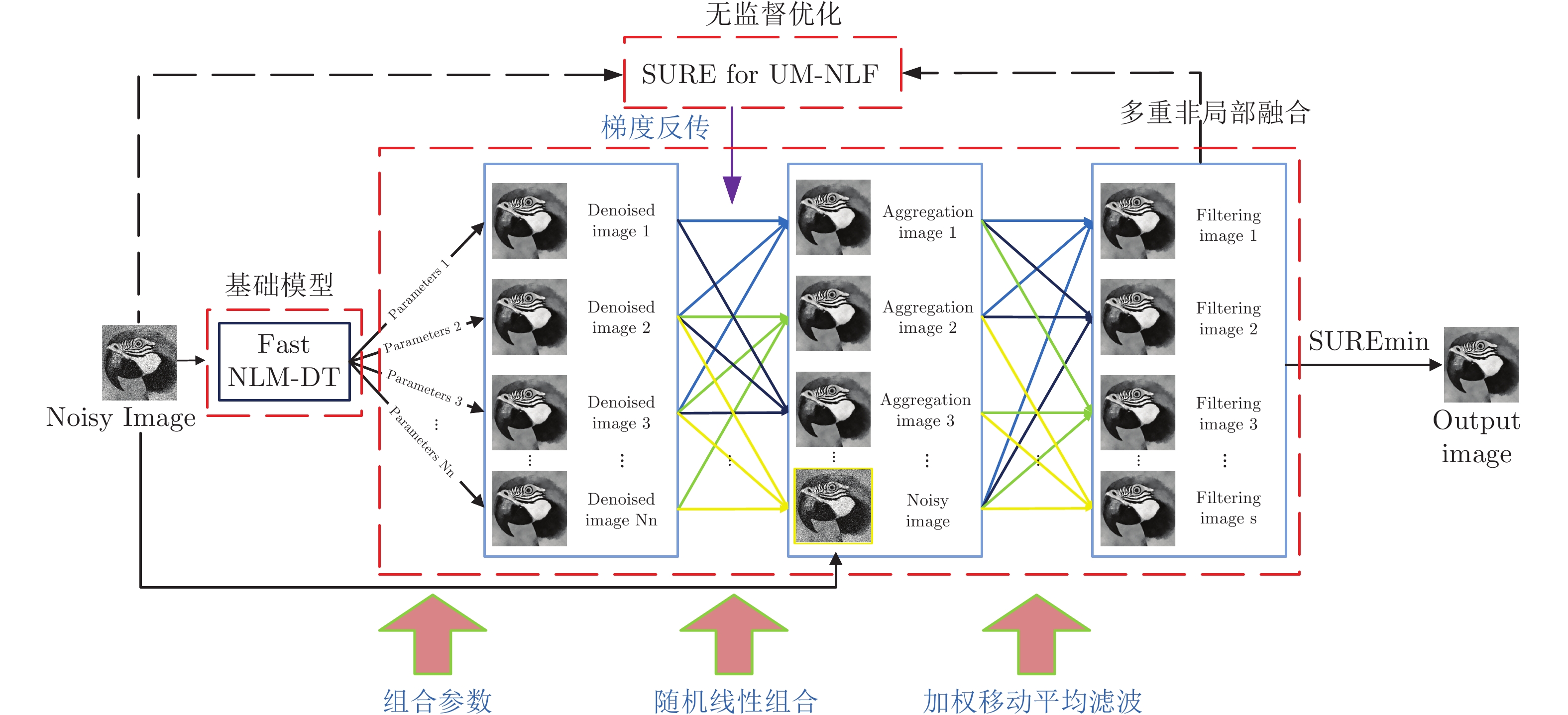
摘要: 非局部均值去噪 (Non-local means, NLM) 算法利用图像的自相似性, 取得了很好的去噪效果. 然而, NLM 算法对图像中不相似的邻域块分配了过大的权重, 此外算法的搜索窗大小和滤波参数等通常是固定的且无法根据图像内容的变化做出自适应的调整. 针对上述问题, 本文提出一种无监督多重非局部融合 (Unsupervised multi-non-local fusion, UM-NLF) 的图像去噪方法, 即变换搜索窗等组合参数得到多个去噪结果, 并利用 SURE (Stein's unbiased risk estimator) 对这些结果进行无监督的随机线性组合以获得最终结果. 首先, 为了滤除不相似或者相似度较低的邻域块, 本文引入一种基于可微分硬阈值函数的非局部均值 (Non-local means with a differential hard threshold function, NLM-DT) 算法, 并结合快速傅里叶变换 (Fast Fourier transformation, FFT), 初步提升算法的去噪效果和速度; 其次, 针对不同的组合参数, 利用快速 NLM-DT 算法串联生成多个去噪结果; 然后, 采用蒙特卡洛随机采样的思想对上述多个去噪结果进行随机的线性组合, 并利用基于 SURE 特征加权的移动平均滤波算法来抑制多个去噪结果组合引起的抖动噪声; 最后, 利用噪声图像和移动平均滤波后图像的 SURE 进行梯度的反向传递来优化随机线性组合的系数. 在公开数据集上的实验结果表明: UM-NLF 算法去噪结果的峰值信噪比 (Peak signal to noise ratio, PSNR) 超过了 NLM 及其大部分改进算法, 以及在部分图像上超过了 BM3D 算法. 同时, UM-NLF 相比于 BM3D 算法在视觉上产生更少的振铃伪影, 改善了图像的视觉质量.Abstract: Non-local means (NLM) denoising algorithm achieves a good denoising effect with the self-similarity of images. However, NLM assigns excessive weights to dissimilar neighborhood patches in the image. Meanwhile the parameters of NLM, such as the search window size, filtering coefficient and so on, are usually fixed and could not make adaptive adjustments based on changes of image content. In view of the above problems, this paper proposes an unsupervised multi-non-local fusion (UM-NLF) image denoising method, transforming the combined parameters such as the search window to obtain multiple denoising results and making an unsupervised stochastic linear combination for these results by using the Stein's unbiased risk estimator (SURE) to obtain the final result. Firstly, in order to eliminate dissimilar or low similarity neighborhood patches, this paper proposes a non-local means with a differentiable hard threshold function (NLM-DT) algorithm, and then combines fast Fourier transformation to make the preliminary improvements in the denoising effect and speed of the algorithm; Secondly, the paper uses a fast NLM-DT algorithm to generate multiple denoising results in series for different combination parameters; Then this paper combines the above multiple denoising results randomly and linearly with the Monte Carlo random sampling, and uses a weighted moving average filtering algorithm based on SURE features to suppress the jitter noise caused by the combination of multiple denoising results; Finally, the paper uses the SURE of the noise image and the filtered image to optimize linear combination unsupervisedly by the back propagation of gradients. Experiments show that the peak signal to noise ratio (PSNR) of UM-NLF algorithm exceeds those of NLM and most of the improved algorithms of NLM on public datasets and exceeds BM3D on some images. Besides, UM-NLF produces fewer ringing artifacts than BM3D algorithm visually, which improves the visual quality of the image.1) 收稿日期 2020-03-16 录用日期 2020-06-11 Manuscript received March 16, 2020; accepted June 11, 2020 国家重点研发计划 (2018TFE0200200), 教育部重大科技创新研究项目, 北京智源人工智能研究院资助 Supported by National Key Research and Development Program of China (2018YFE0200200), Key Scientific Technological Innovation Research Project by Ministry of Education, Beijing Academy of Artificial Intelligence 本文责任编委 黄庆明2) Recommended by Associate Editor HUANG Qing-Ming 1. 西安交通大学电子与信息学部自动化科学与工程学院 西安 710049 2. 清华大学精密仪器系类脑计算研究中心 北京 100084 1. School of Automation Science and Engineering, Faculty of Electronic and Information Engineering, Xi' an Jiaotong University, Xi' an 710049 2. Center for Brain Inspired Computing Research, Department of Precision Instrument, Tsinghua University, Beijing 100084
-
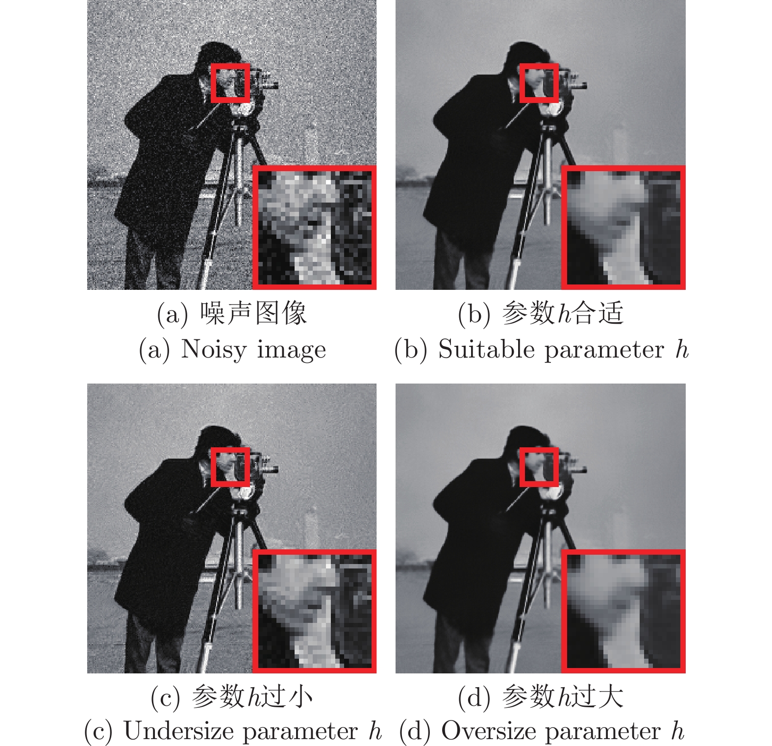
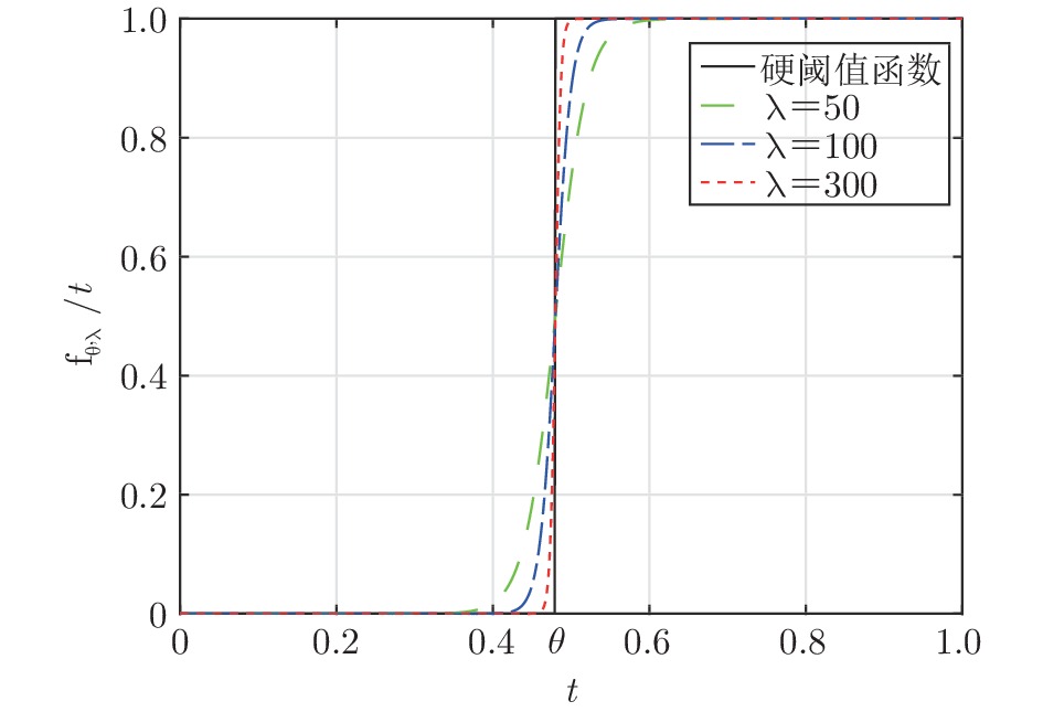
图 2 参数
$ h $ 对算法去噪效果的影响Fig. 2 The effect of parameter
$ h $ on the denoising effect of the algorithm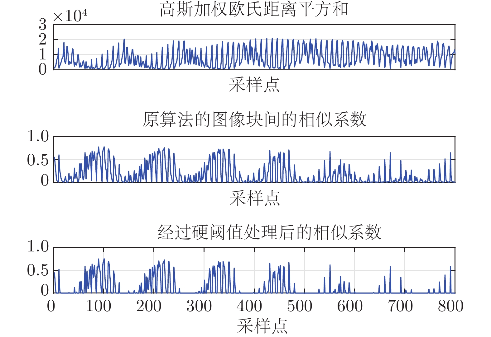
图 4 硬阈值加入前后相似权重值的对比
Fig. 4 Comparisons of similar weight values before and after adding a hard threshold
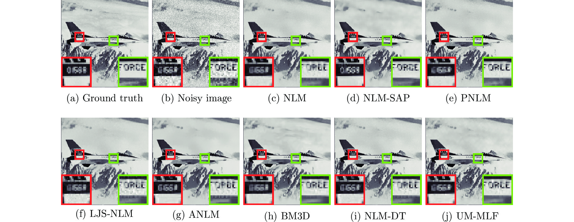
图 6 不同算法对噪声等级
$ \sigma = 20 $ 的Airplane噪声图像的去噪结果PSNR (dB)和SSIM ((a) 原始无失真图像;(b) 噪声图像(22.08 dB/0.4397); (c) NLM (28.33 dB/0.8328); (d) NLM-SAP (28.94 dB/0.8526); (e) PNLM(29.04 dB/0.8490); (f) LJS-NLM (28.37 dB/0.8410); (g) ANLM (27.86 dB/0.8489); (h) BM3D (29.55 dB/0.8755); (i) NLM-DT (28.60 dB/0.8418); (j) UM-NLF (29.83 dB/0.8760))Fig. 6 Denoising results PSNR (dB) and SSIM on noisy image Airplane with noise level
$ \sigma = 20 $ by different methods ((a) Ground truth; (b) Noisy image (22.08 dB/0.4397); (c) NLM (28.33 dB/0.8328); (d) NLM-SAP (28.94 dB/0.8526); (e) PNLM (29.04 dB/0.8490); (f) LJS-NLM (28.37 dB/0.8410); (g) ANLM (27.86 dB/0.8489); (h) BM3D (29.55 dB/0.8755); (i) NLM-DT (28.60 dB/0.8418); (j) UM-NLF (29.83 dB/0.8760))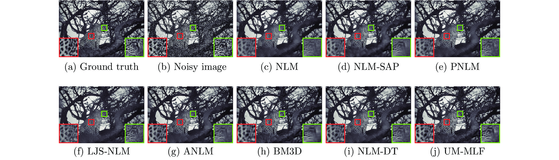
图 7 不同算法对噪声等级
$ \sigma = 35 $ 的“Test016” 噪声图像的去噪结果PSNR (dB)和SSIM ((a) 原始无失真图像;(b) 噪声图像(17.25 dB/0.4201); (c) NLM (24.41 dB/0.7202); (d) NLM-SAP (24.75 dB/0.7293); (e) PNLM(24.85 dB/0.7376); (f) LJS-NLM (23.94 dB/0.7168); (g) ANLM (24.89 dB/0.7540); (h) BM3D(25.48 dB/0.7850); (i) NLM-DT (25.04 dB/0.7422); (j) UM-NLF (25.91 dB/0.7853))Fig. 7 Denoising results PSNR (dB) and SSIM on noisy image “Test016” with noise level
$ \sigma = 35 $ by different methods ((a) Ground truth; (b) Noisy image (17.25 dB/0.4201); (c) NLM (24.41 dB/0.7202); (d) NLM-SAP (24.75 dB/0.7293); (e) PNLM (24.85 dB/0.7376); (f) LJS-NLM (23.94 dB/0.7168); (g) ANLM (24.89 dB/0.7540); (h) BM3D (25.48 dB/0.7850); (i) NLM-DT (25.04 dB/0.7422); (j) UM-NLF (25.91 dB/0.7853))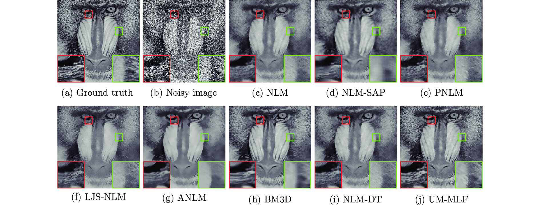
图 8 不同算法对噪声等级
$ \sigma = 50 $ 的Baboon噪声图像的去噪结果PSNR (dB)和SSIM ((a) 原始无失真图像;(b) 噪声图像 (14.16 dB/0.2838); (c) NLM (21.40 dB/0.4674); (d) NLM-SAP (21.33 dB/0.4386); (e) PNLM(21.48 dB/0.4793); (f) LJS-NLM (21.35 dB/0.4866); (g) ANLM (21.40 dB/0.4529); (h) BM3D(22.35 dB/0.5489); (i) NLM-DT (21.62 dB/0.4840); (j) UM-NLF (22.53 dB/0.5739))Fig. 8 Denoising results PSNR (dB) and SSIM on noisy image Baboon with noise level
$ \sigma = 50 $ by different methods ((a) Ground truth; (b) Noisy image (14.16 dB/0.2838); (c) NLM (21.40 dB/0.4674); (d) NLM-SAP (21.33 dB/0.4386); (e) PNLM (21.48 dB/0.4793); (f) LJS-NLM (21.35 dB/0.4866); (g) ANLM (21.40 dB/0.4529); (h) BM3D (22.35 dB/0.5489); (i) NLM-DT (21.62 dB/0.4840); (j) UM-NLF (22.53 dB/0.5739))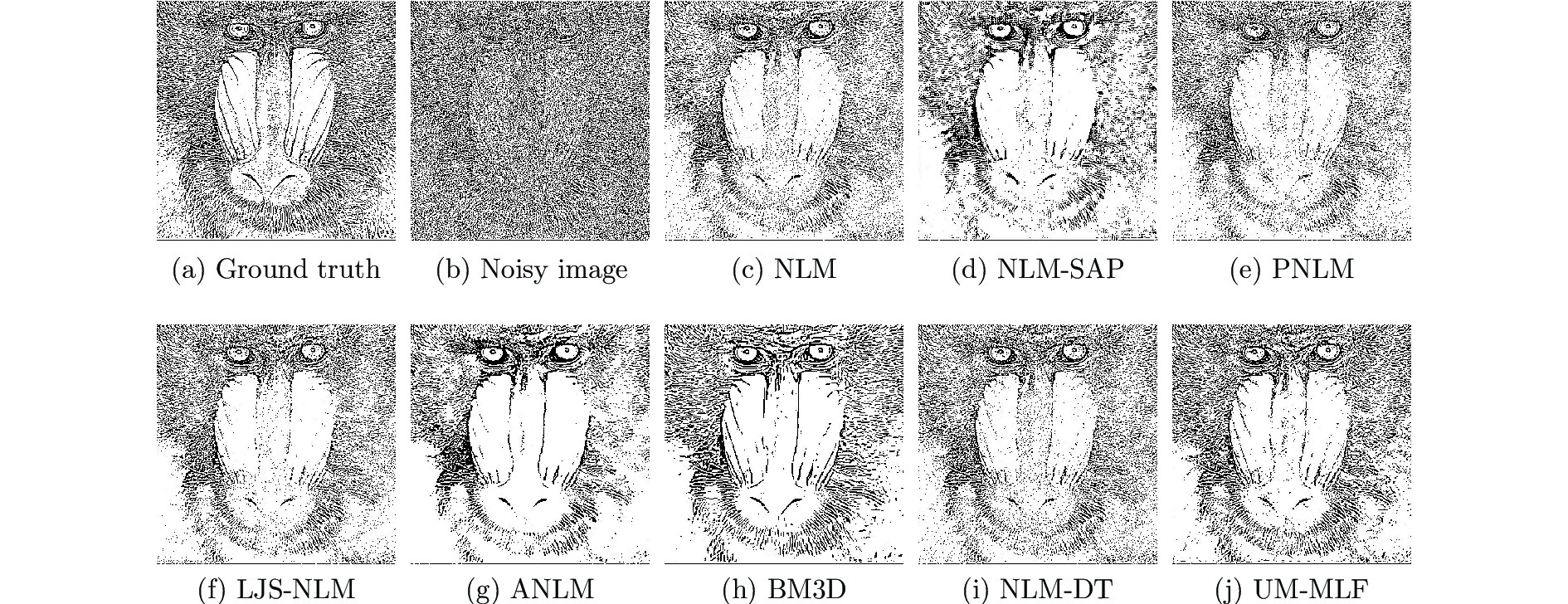
图 9 不同算法对Baboon噪声图像去噪后并经过XDoG滤波的结果
Fig. 9 XDoG filtered results of the denoised images of different algorithms on noisy image Baboon
表 1 UM-NLF算法的参数选择
Table 1 Parameter selection of UM-NLF algorithm
图像大小 参数 参数值 邻域块的直径 $[5, 7, 11]$ 搜索窗的直径 $[13, 21]$ 高斯核的系数 $[1, 2, 4]$ $256\times 256$ 滤波参数 $[0.8, 1.0, 1.2, \cdots, 2.4]$ 硬阈值参数 $[0, 0.02, 0.04]\times \rm exp(-\frac{1}{\sigma^2})$ 线性组合的数目 40 蒙特卡洛的次数 80 加权移动平均的数目 8 邻域块的直径 $[5, 7, 11]$ 搜索窗的直径 $[13, 21]$ 高斯核的系数 $[1, 2, 4]$ $512\times 512$ 滤波参数 $[0.8, 0.95, 1.1,\cdots, 2.3]$ 硬阈值参数 $[0, 0.04, 0.08]\times \rm exp(-\frac{1}{\sigma^2})$ 线性组合的数目 70 蒙特卡洛的次数 150 加权移动平均的数目 8  下载: 导出CSV
表 2 在13张噪声水平
$\sigma$ 分别为10、15、20、25、35和50的噪声图像上不同算法去噪结果的PSNR (dB)Table 2 The PSNR (dB) results of different methods on 13 gray images with noise level
$\sigma$ at 10、15、20、25、35 and 50Level Images C.man House Peppers Starfish Monarch Airplane Parrot Lena Barbara Boat Man Couple Baboon NLM 31.83 35.35 33.23 32.22 32.47 31.02 31.42 34.85 33.80 32.70 32.66 32.59 28.55 NLM-SAP 33.50 35.49 34.20 32.44 33.69 32.86 32.92 35.06 33.77 32.97 33.18 33.08 29.78 PNLM 33.50 35.28 33.66 32.74 33.49 32.85 32.82 34.63 33.39 32.90 33.15 32.78 29.92 LJS-NLM 33.08 35.18 33.27 32.10 32.54 32.23 32.55 34.54 33.56 32.64 32.82 32.56 30.11 $\sigma=10$ ANLM 30.33 34.66 32.05 30.69 30.99 29.44 29.84 34.33 32.73 31.88 32.06 31.86 26.97 BM3D 34.19 36.71 34.68 33.30 34.12 33.33 33.57 35.93 34.98 33.92 33.98 34.04 30.58 NLM-DT 32.06 35.39 33.23 32.05 33.31 31.03 31.53 34.90 33.63 32.87 32.92 32.74 28.64 UM-NLF 34.13 36.07 34.71 33.54 34.34 33.54 33.60 35.70 34.44 33.68 33.98 33.64 30.66 NLM 30.35 33.75 31.35 30.37 30.75 29.59 30.06 32.89 31.67 30.80 30.71 30.49 26.92 NLM-SAP 31.18 33.85 32.24 30.37 31.28 30.54 30.68 33.32 31.93 31.02 31.03 30.94 27.41 PNLM 31.25 33.46 31.40 30.42 31.13 30.58 30.64 32.60 31.06 30.86 30.95 30.45 27.59 LJS-NLM 30.86 33.26 31.05 29.89 30.29 29.93 30.35 32.43 31.19 30.45 30.58 30.11 27.54 $\sigma=15$ ANLM 29.37 33.34 30.83 29.54 29.79 28.65 28.98 32.87 31.32 30.56 30.58 30.47 26.18 BM3D 31.91 34.93 32.69 31.14 31.85 31.07 31.37 34.26 33.10 32.13 31.92 32.10 28.18 NLM-DT 30.55 33.79 31.52 30.34 30.69 29.67 30.12 33.09 31.84 31.08 31.08 30.87 27.18 UM-NLF 31.92 34.47 32.70 31.36 32.12 31.34 31.44 34.01 32.57 31.82 31.95 31.61 28.32 NLM 29.24 32.26 29.86 28.68 29.35 28.33 28.96 31.41 29.91 29.32 29.31 28.79 25.44 NLM-SAP 29.69 32.48 30.77 28.78 29.58 28.94 29.23 31.92 30.38 29.60 29.58 29.31 25.94 PNLM 29.73 31.95 29.79 28.69 29.51 29.04 29.24 31.15 29.27 29.38 29.44 28.76 26.00 LJS-NLM 29.35 31.69 29.43 28.15 28.75 28.37 28.92 30.96 29.38 28.91 29.05 28.34 25.82 $\sigma=20$ ANLM 28.56 32.41 29.65 28.47 28.76 27.86 28.23 31.68 30.12 29.45 29.41 29.25 25.27 BM3D 30.49 33.77 31.29 29.67 30.35 29.55 29.96 33.05 31.78 30.88 30.59 30.76 26.61 NLM-DT 29.37 32.51 30.10 28.97 29.38 28.60 29.01 31.68 30.28 29.70 29.74 29.35 25.97 UM-NLF 30.44 33.29 31.22 29.80 30.61 29.82 30.03 32.77 31.17 30.51 30.59 30.23 26.80 NLM 28.29 30.89 28.62 27.25 28.19 27.27 28.05 30.26 28.49 28.17 28.24 27.46 24.26 NLM-SAP 28.61 31.20 29.55 27.43 28.26 27.75 28.24 30.76 29.05 28.47 28.48 27.98 24.74 PNLM 28.58 30.68 28.52 27.33 28.26 27.83 28.21 30.02 27.85 28.23 28.30 27.46 24.77 LJS-NLM 28.16 30.39 28.11 26.76 27.53 27.16 27.84 29.86 27.95 27.74 27.91 27.04 24.57 $\sigma=25$ ANLM 27.91 31.62 28.66 27.49 27.88 27.07 27.57 30.69 29.05 28.50 28.49 28.16 24.38 BM3D 29.45 32.85 30.16 28.56 29.25 28.42 28.93 32.07 30.71 29.90 29.61 29.71 25.46 NLM-DT 28.47 31.24 28.95 27.72 28.29 27.70 28.11 30.54 28.97 28.64 28.69 28.10 24.97 UM-NLF 29.35 32.29 30.04 28.56 29.42 28.67 29.00 31.79 30.07 29.51 29.56 29.12 25.69 NLM 26.57 28.64 26.66 25.16 26.30 25.48 26.58 28.53 26.35 26.44 26.67 25.67 22.69 NLM-SAP 26.88 28.88 27.47 25.27 26.30 25.76 26.70 28.94 26.90 26.72 26.89 26.06 22.89 PNLM 26.76 28.56 26.54 25.32 26.34 25.86 26.65 28.28 25.76 26.47 26.62 25.66 23.02 LJS-NLM 26.19 28.22 26.11 24.75 25.58 25.16 26.22 28.20 25.86 26.01 26.30 25.30 22.86 $\sigma=35$ ANLM 26.82 30.05 27.16 25.76 26.43 25.79 26.46 29.16 27.24 26.97 27.11 26.31 22.86 BM3D 27.92 31.36 28.51 26.86 27.58 26.83 27.40 30.56 28.98 28.43 28.22 28.15 23.82 NLM-DT 26.98 29.05 27.03 25.65 26.54 26.01 26.73 28.76 26.85 26.91 27.03 26.15 23.38 UM-NLF 27.77 30.64 28.26 26.70 27.70 26.86 27.54 30.22 28.42 27.96 28.07 27.45 24.09 NLM 24.39 26.14 24.48 23.17 24.00 23.36 24.82 26.61 24.26 24.65 25.07 24.06 21.40 NLM-SAP 24.75 26.32 25.10 23.14 24.07 23.37 24.95 27.07 24.63 24.94 25.36 24.39 21.33 PNLM 24.67 25.96 24.23 23.17 23.99 23.54 24.84 26.34 23.71 24.61 24.89 23.96 21.48 LJS-NLM 24.06 25.79 23.84 22.83 23.31 23.06 24.38 26.34 23.83 24.30 24.70 23.71 21.35 $\sigma=50$ ANLM 25.43 27.95 25.44 23.84 24.82 24.24 25.21 27.61 25.19 25.36 25.69 24.53 21.40 BM3D 26.13 29.69 26.68 25.04 25.82 25.10 25.90 29.05 27.22 26.78 26.81 26.46 22.35 NLM-DT 25.08 26.62 24.94 23.69 24.49 24.02 25.04 26.79 24.65 25.05 25.30 24.38 21.81 UM-NLF 26.06 28.57 26.29 24.80 25.85 24.99 26.04 28.51 26.58 26.31 26.52 25.71 22.53 注: 最佳的两个结果分别以粗体和斜体突出显示
下载: 导出CSV
表 3 不同算法在BSD68灰度数据集上的平均PSNR (dB)和SSIM
Table 3 Average PSNR (dB) and SSIM results of different methods on BSD68 gray dataset
$\sigma$ NLM NLM-SAP PNLM LJS-NLM ANLM BM3D NLM-DT UM-NLF 10 31.37/0.8809 32.47/0.9006 32.52/0.9000 32.30/0.8984 30.72/0.8834 33.32/0.9163 31.57/0.8934 33.35/0.9184 15 29.64/0.8281 30.29/0.8472 30.25/0.8472 29.95/0.8448 29.44/0.8412 31.07/0.8720 29.96/0.8464 31.16/0.8760 20 28.31/0.7803 28.84/0.7973 28.73/0.7994 28.38/0.7967 28.41/0.8029 29.62/0.8342 28.72/0.8015 29.70/0.8367 25 27.28/0.7368 27.75/0.7550 27.60/0.7563 27.22/0.7539 27.56/0.7685 28.57/0.8017 27.73/0.7585 28.64/0.8034 35 25.75/0.6602 26.17/0.6854 25.95/0.6812 25.58/0.6814 26.25/0.7099 27.08/0.7482 26.20/0.6767 27.12/0.7451 50 24.20/0.5643 24.59/0.6069 24.29/0.5893 23.99/0.5945 24.88/0.6403 25.62/0.6869 24.52/0.5685 25.63/0.6768
下载: 导出CSV
表 4 不同算法在大小为
$256\times 256$ 灰度噪声图像上的去噪时间(秒)Table 4 Denoising time (seconds) of different algorithms on gray noisy images with a size of
$ 256\times 256$ $\sigma$ NLM NLM-SAP PNLM LJS-NLM ANLM BM3D NLM-DT UM-NLF 10 71.74$\pm$0.82 10.89$\pm$0.21 7.39$\pm$0.64 1.41$\pm$0.01 6.35$\pm$0.34 0.67$\pm$0.09 68.49$\pm$1.45 25.55$\pm$0.59 15 72.85$\pm$3.45 11.11$\pm$0.20 7.79$\pm$0.58 1.41$\pm$0.03 6.31$\pm$0.04 0.68$\pm$0.09 60.01$\pm$1.42 24.41$\pm$1.23 20 72.58$\pm$4.34 11.23$\pm$0.15 8.09$\pm$0.46 1.40$\pm$0.02 6.25$\pm$0.08 0.70$\pm$0.09 70.68$\pm$0.86 25.27$\pm$1.56 25 72.76$\pm$1.62 11.36$\pm$0.10 8.37$\pm$0.58 1.40$\pm$0.01 6.26$\pm$0.20 0.68$\pm$0.11 64.71$\pm$2.45 24.98$\pm$3.12 35 71.68$\pm$0.70 11.43$\pm$0.12 8.74$\pm$0.31 1.39$\pm$0.03 6.25$\pm$0.13 0.67$\pm$0.10 60.40$\pm$0.78 24.68$\pm$2.32 50 71.48$\pm$1.07 11.48$\pm$0.05 8.95$\pm$0.40 1.39$\pm$0.01 6.27$\pm$0.19 0.87$\pm$0.05 62.52$\pm$1.45 24.30$\pm$1.22
下载: 导出CSV
表 5 不同算法在大小为
$512\times 512$ 灰度噪声图像上的去噪时间(秒)Table 5 Denoising time (seconds) of different algorithms on gray noisy images with a size of
$512\times 512$ $\sigma$ NLM NLM-SAP PNLM LJS-NLM ANLM BM3D NLM-DT UM-NLF 10 284.37$\pm$13.82 66.46$\pm$0.66 38.48$\pm$3.46 10.37$\pm$0.40 25.27$\pm$0.65 3.16$\pm$0.13 281.63$\pm$11.13 155.64$\pm$8.90 15 282.18$\pm$11.25 67.77$\pm$2.22 41.25$\pm$3.55 10.30$\pm$0.33 25.46$\pm$0.68 3.26$\pm$0.11 281.31$\pm$10.23 160.28$\pm$5.34 20 285.50$\pm$11.34 68.70$\pm$1.82 42.85$\pm$2.50 10.15$\pm$0.49 25.70$\pm$0.66 3.32$\pm$0.11 287.31$\pm$13.33 155.94$\pm$9.91 25 283.65$\pm$12.72 69.53$\pm$0.63 44.46$\pm$4.01 10.18$\pm$0.31 25.54$\pm$0.32 3.33$\pm$0.08 275.43$\pm$14.23 151.56$\pm$5.23 35 284.15$\pm$15.70 70.41$\pm$0.60 46.88$\pm$1.89 10.21$\pm$0.25 25.40$\pm$0.71 3.20$\pm$0.17 279.51$\pm$13.32 150.65$\pm$4.43 50 279.63$\pm$19.07 71.46$\pm$2.11 49.37$\pm$2.83 10.36$\pm$0.18 25.40$\pm$0.49 3.86$\pm$0.09 289.26$\pm$14.24 158.75$\pm$6.45
下载: 导出CSV
表 6 传统算法和深度学习算法在BSD68灰度数据集上的平均PSNR (dB)和SSIM
Table 6 Average PSNR (dB) and SSIM results of traditional and deep learning methods on BSD68 gray dataset
传统的无监督去噪方法 无监督式神经网络去噪方法 有监督式神经网络去噪方法 $\sigma$ BM3D UM-NLF Noise2Void GCBD TNRD DnCNN-S 15 31.07/0.8720 31.16/0.8760 −/− 31.59/− 31.42/0.8822 31.73/0.8906 25 28.57/0.8017 28.64/0.8034 27.71/− 29.15/− 28.92/0.8148 29.23/0.8278 50 25.62/0.6869 25.62/0.6762 −/− −/− 25.97/0.7021 26.23/0.7189 注: “−”表示原始论文中没有给出相应的实验结果
下载: 导出CSV
-
[1] Tian C W, Fei L K, Zheng W X, Xu Y, Zuo W M, Lin C W. Deep learning on image denoising: an overview [online], available: http://arxiv.org/abs/1912.13171, January 16, 2020 [2] Dong W S, Wang P Y, Yin W T, Shi G M, Wu F F, Lu X T. Denoising prior driven deep neural network for image restoration. IEEE Transactions on Pattern Analysis and Machine Intelligence, 2019, 41(10): 2305−2318 doi: 10.1109/TPAMI.2018.2873610 [3] Geman S, Geman D. Stochastic relaxation, gibbs distributions, and the bayesian restoration of images. IEEE Transactions on Pattern Analysis and Machine Intelligence, 1984, 6(5-6): 721−741 [4] Buades A, Coll B, Morel J M. A non-local algorithm for image denoising. In: Proceedings of the 2005 IEEE Computer Society Conference on Computer Vision and Pattern Recognition. San Diego, California, USA: IEEE, 2005.60−65 [5] Mahmoudi M, Sapiro G. Fast image and video denoising via non-local means of similar neighborhoods. IEEE Signal Processing Letters, 2005, 12(12), 839−842 doi: 10.1109/LSP.2005.859509 [6] Coupe P, Yger P, Prima S, Hellier P, Kervrann C, Barillot C. An optimized blockwise nonlocal means denoising filter for 3-D magnetic resonance images. IEEE Transactions on Medical Imaging, 2008, 27(4), 425−441 doi: 10.1109/TMI.2007.906087 [7] Vignesh R, Oh B T, Kuo C C J. Fast non-local means (NLM) computation with probabilistic early termination. IEEE Signal Processing Letters, 2010, 17(3), 277−280 doi: 10.1109/LSP.2009.2038956 [8] Tasdizen T. Principal neighborhood dictionaries for nonlocal means image denoising. IEEE Transactions on Image Processing, 2009, 18(12): 2649−2660 doi: 10.1109/TIP.2009.2028259 [9] Chan S H, Zickler T, Lu Y M. Monte carlo non-local means: random sampling for large-scale image filtering. IEEE Transactions on Image Processing, 2014, 23(8): 3711−3725 doi: 10.1109/TIP.2014.2327813 [10] Karam C, Hirakawa K. Monte-carlo acceleration of bilateral filter and non-local means. IEEE Transactions on Image Processing, 2018, 27(3): 1462−1474 doi: 10.1109/TIP.2017.2777182 [11] Wang J, Guo Y W, Ying Y T, Liu Y L, Peng Q S. Fast nonlocal algorithm for image denoising. In: Proceedings of the 2006 IEEE International Conference on Image Processing. Atlanda, GA, USA: IEEE, 2006.1429−1432 [12] Chaudhury K N, Singer A. Non-local euclidean medians. IEEE Signal Processing Letters, 2012, 19(11), 745−748 doi: 10.1109/LSP.2012.2217329 [13] Wu Y, Tracey B, Natarajan P, Noonan J P. Probabilistic non-local means. IEEE Signal Processing Letters, 2013, 20(8), 763−766 doi: 10.1109/LSP.2013.2263135 [14] Deledalle C A, Duval V, Salmon J. Non-local methods with shape-adaptive patches (NLM-SAP). Journal of Mathematical Imaging and Vision, 2012, 43(2): 103−120 doi: 10.1007/s10851-011-0294-y [15] Grewenig S, Zimmer S, Weickert J. Rotationally invariant similarity measures for nonlocal image denoising. Journal of Visual Communication and Image Representation, 2011, 22(2): 117−130 doi: 10.1016/j.jvcir.2010.11.001 [16] Wu Y, Tracey B, Natarajan P, Noonan J P. James-stein type center pixel weights for non-local means image denoising. IEEE Signal Processing Letters, 2013, 20(4), 411−414 doi: 10.1109/LSP.2013.2247755 [17] Nguyen M P, Chun S Y. Bounded self-weights estimation method for non-local means image denoising using minimax estimators. IEEE Transactions on Image Processing, 2017, 26(4): 1637−1649 doi: 10.1109/TIP.2017.2658941 [18] Salmon J. On two parameters for denoising with nonlocal means. IEEE Signal Processing Letters, 2010, 17(3), 269−272 doi: 10.1109/LSP.2009.2038954 [19] Van D V D, Kocher M. SURE-based non-local means. IEEE Signal Processing Letters, 2009, 16(11), 973−976 doi: 10.1109/LSP.2009.2027669 [20] Stein C M. Estimation of the mean of a multivariate normal distribution. The Annals of Statistics, 1981, 9(6), 1135−1151 doi: 10.1214/aos/1176345632 [21] Dong W S, Zhang L, Shi G M, Li X. Nonlocally centralized sparse representation for image restoration. IEEE Transactions on Image Processing, 2013, 22(4): 1620−1630 doi: 10.1109/TIP.2012.2235847 [22] May V, Keller Y, Sharon N, Shkolnisky Y. An algorithm for improving non-local means operators via low-rank approximation. IEEE Transactions on Image Processing, 2016, 25(3): 1340−1353 doi: 10.1109/TIP.2016.2518805 [23] Dabov K, Foi A, Katkovnik V, Egiazarian K. Image denoising by sparse 3-D transform-domain collaborative filtering. IEEE Transactions on Image Processing, 2007, 16(8): 2080−2095 doi: 10.1109/TIP.2007.901238 [24] Li X Y, Zhou Y C, Zhang J, Wang L H. Multipatch unbiased distance non-local adaptive means with wavelet shrinkage. IEEE Transactions on Image Processing, 2020, 29: 157−169 doi: 10.1109/TIP.2019.2928644 [25] Wan L, Zeiler M D, Zhang S, Yann L C, Fergus R. Regularization of neural networks using dropconnect. In: Proceedings of the 2013 IEEE International Conference on Machine Learning. Atlanta, GA, USA: IEEE, 2013.1058−1066 [26] 邢笑笑, 王海龙, 李健, 张选德. 渐近非局部平均图像去噪算法. 自动化学报, 2020, 46(9): 1952−1960Xing Xiao-Xiao, Wang Hai-Long, Li Jian, Zhang Xuan-De. Asymptotic non-local means image denoising algorithm. Acta Automatica Sinica, 2020, 46(9): 1952−1960 [27] Chen Y J, Pock T. Trainable nonlinear reaction diffusion: a flexible framework for fast and effective image restoration. IEEE Transactions on Pattern Analysis and Machine Intelligence, 2017, 39(6): 1256−1272 doi: 10.1109/TPAMI.2016.2596743 [28] Zhang K, Zuo W M, Chen Y J, Meng D Y, Zhang L. Beyond a gaussian denoiser: residual learning of deep CNN for image denoising. IEEE Transactions on Image Processing, 2017, 26(7): 3142−3155 doi: 10.1109/TIP.2017.2662206 [29] Chen J W, Chen J W, Cao H Y, Yang M. Image blind denoising with generative adversarial network based noise modeling. In: Proceedings of the 2018 IEEE Conference on Computer Vision and Pattern Recognition. Salt Lake City, Utah, USA: IEEE, 2018. 3155−3164 [30] Krull A, Buchholz T O, Jug F. Noise2Void-learning denoising from single noisy images. In: Proceedings of the 2019 IEEE Conference on Computer Vision and Pattern Recognition. Long Beach, CA, USA: IEEE, 2019. 2129−2137 [31] Roth S, Black M J. Fields of experts. International Journal of Computer Vision, 2009, 82(2): 205−229 doi: 10.1007/s11263-008-0197-6 [32] Wang Z, Bovik A C, Sheikh H R, Simoncelli E P. Image quality assessment: from error visibility to structural similarity. IEEE Transactions on Image Processing, 2004, 13(4): 600−612 doi: 10.1109/TIP.2003.819861 [33] Winnemoller H, Kyprianidis J E, Olsen S C. XDoG: an extended difference-of-gaussians compendium including advanced image stylization. Computers & Graphics, 2012, 36(6): 740−753 -

 下载:
下载:


计量
- 文章访问数: 2047
- HTML全文浏览量: 941
- PDF下载量: 493
- 被引次数: 0
