

Probabilistic Multimodal Optimization Algorithm Based on the Buffon Distance in Noisy Environment
-
摘要: 针对噪声环境下求解多个极值点的问题, 本文提出了噪声环境下基于蒲丰距离的依概率多峰优化算法(Probabilistic multimodal optimization algorithm based on the Button distance, PMB). 算法依据蒲丰投针原理提出噪声下的蒲丰距离和极值分辨度概念, 理论推导证明了二者与算法峰值检测率符合依概率关系. 在全局范围内依据蒲丰距离划分搜索空间, 可以使PMB算法保持较好的搜索多样性. 在局部范围内利用改进的斐波那契法进行探索, 减少了算法陷入噪声引起的局部最优的概率. 基于34个测试函数, 从依概率特性验证、寻优结果影响因素分析、多极值点寻优和多维函数寻优四个角度进行实验. 证明了蒲丰距离与算法的峰值检测率符合所推导的依概率关系. 对比噪声环境下的改进蝙蝠算法和粒子群算法, PMB算法在噪声环境中可以依定概率更精确地定位多峰函数的更多极值点, 从而证明了PMB算法原理的正确性和噪声条件下全局寻优的依概率性能, 具有理论意义和实用价值.Abstract: To solve the problem of multiple extremum points optimization in noisy environment, a probabilistic multimodal optimization algorithm based on the Buffon distance (PMB) is proposed in this paper. Based on the principle of Buffon needles, the concepts of Buffon distance and resolution of extreme value under noisy environment are put forward. The theoretical derivation proves that the relationship between peak detection rate of PMB algorithm and Buffon distance conforms to a probabilistic relation. In global scope, the search space is divided by Buffon distance for diversity maintenance. The improved Fibonacci method is used in local search to reduce the probability of falling into the local optimum caused by noise. Based on 34 test functions, experiments are carried out from four aspects, including probabilistic property verification, analysis of influencing factors of optimization results, multiple extremum points optimization and multidimensional optimization. It is proved that the relationship of Buffon distance and peak detection rate of PMB algorithm is in line with the deduced probabilistic relationship. Compared with the improved bat algorithm and particle swarm optimization (PSO), PMB algorithm can locate extremum points of multimodal function by a steady probability in noise environment, and gain more extremum points accurately. Thus, the correctness of PMB algorithm principle and probabilistic performance of global optimization under noise condition are proved, which has theoretical and practical significance.
-
Key words:
- Noisy environment /
- multimodal optimization /
- Buffon distance /
- probabilistic
1) 收稿日期 2019-07-01 录用日期 2019-11-16 Manuscript received July 1, 2019; accepted November 16, 2019 国家自然科学基金(61763046, 61762093, 61662089, 61761048), 云南省第十七批中青年学术和技术带头人资助项目 (2014HB019), 云南省高校科技创新团队支持计划资助, 云南省教育厅科学研究基金(2017ZZX229), 云南省应用基础研究重点项目 (2018FA036) 资助 Supported by National Natural Science Foundation of China (61763046, 61762093, 61662089, 61761048), The 17th Batches of Young and Middle-aged Leaders in Academic and Technical Reserved Talents Project of Yunnan Province (2014HB019), The Program for Innovative Research Team (in Science and Technology) in University of Yunnan Province, Yunnan Provincial Department of Education Science Research Fund Project (2017ZZX229),2) and Key Projects of Applied Basic Research of Yunnan Province (2018FA036) 本文责任编委 穆朝絮 Recommended by Associate Editor MU Chao-Xu 1. 云南大学信息学院 昆明 650500 2. 云南民族大学电气信息工程学院 昆明 650500 1. School of Information Science and Engineering, Yunnan University, Kunming 650500 2. School of Electrical and Informa-tion Engineering, Yunnan Minzu University, Kunming 650500 -

图 5 蒲丰距离与针长的关系示意图
Fig. 5 Diagram of the relationship between Buffon distance and needle length
图 6 改进的斐波那契法的区域伸缩过程
Fig. 6 The process of regional scaling of the improved Fibonacci method
图 9
$a$ = 0.2时无噪声环境下PMB算法对TF1中的$f_1$ 的寻优结果Fig. 9 Optimization results for
$f_1$ of TF1 by PMB algorithm in noiseless environment with$a$ = 0.2
图 14
$\sigma^2$ = 0.01,$a$ = 0.2时PMB算法对TF1中的$f_1$ 的寻优结果Fig. 14 Optimization results for
$f_1$ of TF1 by PMB algorithm in noise environment with$\sigma^2$ = 0.01 and$a$ = 0.2
图 11
$\sigma^2$ = 0.05,$a$ = 0.5时PMB算法对TF1中的$f_1$ 的寻优结果Fig. 11 Optimization results for
$f_1$ of TF1 by PMB algorithm in noise environment with$\sigma^2$ = 0.05 and$a$ = 0.5
图 10
$a$ = 0.5时无噪声环境下PMB算法对TF1中的$f_1$ 的寻优结果Fig. 10 Optimization results for
$f_1$ of TF1 by PMB algorithm in noiseless environment with$a$ = 0.5
图 12
$\sigma^2$ = 0.01,$a$ = 0.5时PMB算法对TF1中的$f_1$ 的寻优结果Fig. 12 Optimization results for
$f_1$ of TF1 by PMB algorithm in noise environment with$\sigma^2$ = 0.01 and$a$ = 0.5
图 13
$\sigma^2$ = 0.05,$a$ = 0.2时PMB算法对TF1中的$f_1$ 的寻优结果Fig. 13 Optimization results for
$f_1$ of TF1 by PMB algorithm in noise environment with$\sigma^2$ = 0.05 and$a$ = 0.2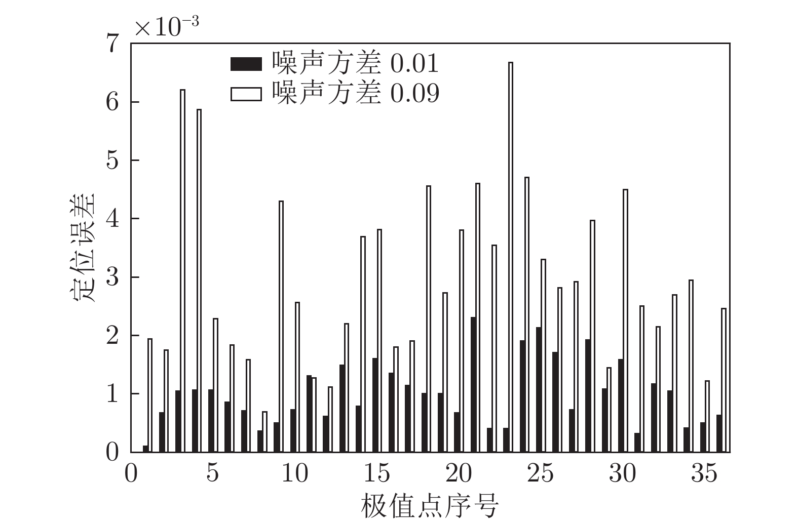
图 15
$a$ = 0.2, PMB算法在不同噪声环境下对TF1中的$f_1$ 求解所有极值点的定位误差Fig. 15 Positioning errors of total-extremum points for
$f_1$ of TF1 searched by PMB algorithm with$a$ = 0.2 under different noise environments
图 16
$a$ = 1,$\sigma^2$ = 0.05, PMB算法对TF1中$f_2$ 的寻优结果Fig. 16 Optimization results for
$f_2$ of TF1 by PMB algorithm in noise environment with$\sigma^2$ = 0.05 and$a$ = 1表 1 测试函数集1 (TF1)
Table 1 Test function set 1 (TF1)
函数 名称 定义域 全局最优值f (与之对应的最优解$\rm{x}_1 $,$ \rm{x}_2$) 表达式 $f_1$ [−1, 1] 3.5326 ($\pm $0.8781, $\pm $0.8781) ${{f}_{1}} = x_{1}^{2}+x_{2}^{2}-\cos(18{{x}_{1}})-\cos (18{{x}_{2}})$ $f_2$ Levy 05 [−10, 10] −176.1375 (−1.3068, −1.4248) $\begin{aligned} {f}_{2}=\;& \sum\nolimits_{i = 1}^{5}{i\cos [(i-1){{x}_{1}}}+i]\times \sum\nolimits_{j = 1}^{5}{j\cos [(j+1){{x}_{2}}+j]}+ \\&{{({{x}_{1}}+1.42513)}^{2}}+{{({{{x}}_{2}}+0.80032)}^{2}}\end{aligned}$ $f_3$ Michalewics [0, ${\text{π}}$] −1.8013 (2.2031, 1.5709) ${{f}_{3}} = -\displaystyle\sum\nolimits_{i = 1}^{2}{\sin ({{x}_{i}})}{{\left(\sin \left(i\times x_{i}^{2}/{\text{π}} \right)\right)}^{20}}$ $f_4$ Periodic [0, ${\text{π}}$] 0.9 (0,0) ${{f}_{4}} = 1+{{\sin }^{2}}({{x}_{1}})+{{\sin }^{2}}({{x}_{2}})-0.1{{ \rm{e}}^{-(x_{1}^{2}+x_{2}^{2})}}$ $f_5$ Carrom Table [−10, 10] −24.1568 ($\pm $9.6466, 9.6466) ${ {f}_{5} } = -\left[{\left\{\cos ({ {x}_{1} })\cos({ {x}_{2} }){ { \rm{e} }^{\left| 1-\sqrt{x_{1}^{2}+x_{2}^{2} }/{\text{π} } \right|} }\right\} }^{2}\right]/30$ $f_6$ Holder Table 2 [−10, 10] −19.2085 ($\pm $8.0550, $\pm $9.6646) ${ {f}_{6} } = -\left| \sin ({ {x}_{1} })\cos ({ {x}_{2} }){ { \rm{e} }^{\left| 1-\sqrt{ { {x}_{1} }+{ {x}_{2} } }/{\text{π} } \right|} } \right|$  下载: 导出CSV
表 2 测试函数集2 (TF2) (维度为5)
Table 2 Test function set 2 (TF2) (Dimension is 5)
函数 全局最优值$f_{i}^{*}$ 函数名称 单峰函数 $f_1$ −1 400 Sphere function $f_2$ −1 300 Rotated high conditioned elliptic function $f_3$ −1 200 Rotated bent cigar function $f_4$ −1 100 Rotated discus function $f_5$ −1 000 Different powers function 多峰函数 $f_6$ −900 Rotated Rosenbrock's function $f_7$ −800 Rotated Schaffers F7 function $f_8$ −700 Rotated Ackley's function $f_9$ −600 Rotated Weierstrass function $f_{10}$ −500 Rotated Griewank's function $f_{11}$ −400 Rastrigin's function $f_{12}$ −300 Rotated Rastrigin's function $f_{13}$ −200 Non-continuous rotated Rastrigin's function $f_{14}$ −100 Schwefel's function $f_{15}$ 100 Rotated Schwefel's function $f_{16}$ 200 Rotated Katsuura function $f_{17}$ 300 Lunacek bi_Rastrigin function $f_{18}$ 400 Rotated lunacek bi_Rastrigin function $f_{19}$ 500 Expanded Griewank's plus Rosenbrock's function $f_{20}$ 600 Expanded Scaffer's F6 function 组合函数 $f_{21}$ 700 Composition function 1 (n = 5, Rotated) $f_{22}$ 800 Composition function 2 (n = 3, Unrotated) $f_{23}$ 900 Composition function 3 (n = 3, Rotated) $f_{24}$ 1 000 Composition function 4 (n = 3, Rotated) $f_{25}$ 1 100 Composition function 5 (n = 3, Rotated) $f_{26}$ 1 200 Composition function 6 (n = 5, Rotated) $f_{27}$ 1 300 Composition function 7 (n = 5, Rotated) $f_{28}$ 1 400 Composition function 8 (n = 5, Rotated)
下载: 导出CSV
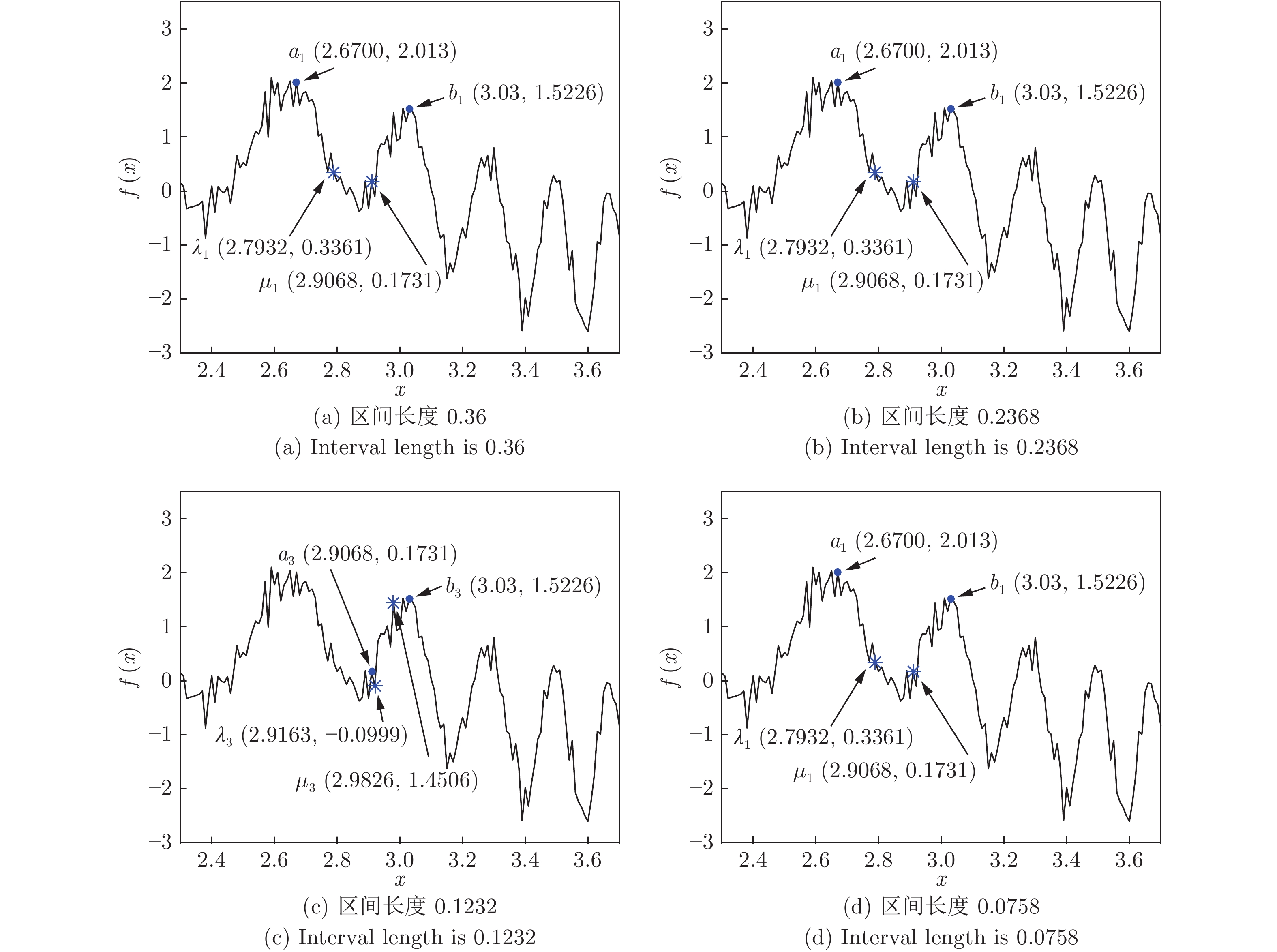
表 3 针对TF1中的
$f_1$ 取不同蒲丰距离时PMB算法在不同噪声环境下的优化结果Table 3 Optimization results of PMB algorithm for
$f_1$ of TF1 in different noise environments with different Buffon distances$\sigma^2$ $a$ Num_mean Num_max Num_min $\eta\_{\rm{mean}}$ $\eta\_{\rm{global}}$ 50 次 0.01 0.5 29.62 33 26 82.28 % 100.00 % 0.2 36.04 37 36 100.11 % 100.00 % 0.05 0.5 31.32 35 27 87.00 % 100.00 % 0.2 36.26 38 36 100.72 % 100.00 % 100 次 0.01 0.5 29.78 33 27 82.72 % 100.00 % 0.2 36.02 37 36 100.06 % 100.00 % 0.05 0.5 32.08 36 28 89.11 % 100.00 % 0.2 36.37 38 36 101.03 % 100.00 % 200 次 0.01 0.5 29.715 34 23 82.54 % 100.00 % 0.2 36.02 37 36 100.06 % 100.00 % 0.05 0.5 32 35 26 88.89 % 100.00 % 0.2 36.4 40 36 101.11 % 100.00 %
下载: 导出CSV
表 4
$a$ = 0.2时PMB算法针对TF1中的$f_1$ 在不同噪声环境下的全局极值点优化数值结果Table 4 Numerical results of global extremum points for
$f_1$ of TF1 searched by PMB algorithm with$a$ = 0.2 under different noise environments极值点序号 P-MQHOA[1] 无噪声 PMB $\sigma^2$ = 0.01 $\sigma^2$ = 0.05 $x_1$ $x_2$ $f$ $x_1$ $x_2$ $f$ $P_f$ $P_l$ $x_1$ $x_2$ $f$ $P_f$ $P_l$ 1 −0.8781 −0.8781 3.5326 −0.8781 −0.878 3.8057 2.73 × 10⁻¹ 1.42 × 10⁻⁴ −0.8776 −0.8773 4.1956 6.63 × 10⁻¹ 9.37 × 10⁻⁴ 2 −0.8781 0.8781 3.5326 −0.8789 0.8784 3.8027 2.70 × 10⁻¹ 7.86 × 10⁻⁴ −0.8788 0.8782 4.1974 6.65 × 10⁻¹ 8.19 × 10⁻⁴ 3 0.8781 −0.8781 3.5326 0.8782 −0.8778 3.8086 2.76 × 10⁻¹ 3.64 × 10⁻⁴ 0.8788 −0.8784 4.2048 6.72 × 10⁻¹ 7.36 × 10⁻⁴ 4 0.8781 0.8781 3.5326 0.8783 0.8775 3.8049 2.72 × 10⁻¹ 6.60 × 10⁻⁴ 0.8774 0.8765 4.2050 6.72 × 10⁻¹ 1.79 × 10⁻³
下载: 导出CSV
表 5
$a$ = 0.5时PMB算法针对TF1中的$f_1$ 在不同噪声环境下的全局极值点优化数值结果Table 5 Numerical results of global extremum points for
$f_1$ of TF1 searched by PMB algorithm with$a$ = 0.5 under different noise environments极值点
序号P-MQHOA[1] 无噪声 PMB $\sigma^2$ = 0.01 $\sigma^2$ = 0.05 $x_1$ $x_2$ $f$ $x_1$ $x_2$ $f$ $P_f$ $P_l$ $x_1$ $x_2$ $f$ $P_f$ $P_l$ 1 −0.8781 −0.8781 3.5326 −0.8760 −0.8780 3.6923 1.60 × 10⁻¹ 2.07 × 10⁻³ −0.8805 −0.8775 3.9568 4.24 × 10⁻¹ 2.46 × 10⁻³ 2 −0.8781 0.8781 3.5326 −0.8771 0.8782 3.6953 1.63 × 10⁻¹ 1.03 × 10⁻³ −0.8770 0.8803 3.9510 4.18 × 10⁻¹ 2.50 × 10⁻³ 3 0.8781 −0.8781 3.5326 0.8775 −0.8794 3.6847 1.52 × 10⁻¹ 1.05 × 10⁻³ 0.8772 −0.8788 3.9467 4.14 × 10⁻¹ 1.14 × 10⁻³ 4 0.8781 0.8781 3.5326 0.8788 0.8784 3.6917 1.59 × 10⁻¹ 8.18 × 10⁻⁴ 0.8775 0.8756 3.9697 4.37 × 10⁻¹ 2.52 × 10⁻³
下载: 导出CSV
表 6 P-MQHOA[1]算法与
$a$ = 0.2时的PMB算法针对TF1中的$f_1$ 在不同环境下的所有极值点求解结果对比Table 6 Comparison of total-extremum points for
$f_1$ of TF1 searched by P-MQHOA[1] algorithm and PMB algorithm with$a$ = 0.2 under different noise environments极值点序号 P-MQHOA[1] 无噪声 PMB $\sigma^2$ = 0.01 $\sigma^2$ = 0.09 $x_1$ $x_2$ $f(x_1,x_2)$ $x_1$ $x_2$ $f(x_1,x_2)$ $x_1$ $x_2$ $f(x_1,x_2)$ 1 −0.8781 −0.8781 3.5326 −0.8781 −0.8780 3.8057 −0.8762 −0.8777 4.4627 2 −0.8781 −0.5269 3.0421 −0.8778 −0.5263 3.3069 −0.8774 −0.5285 3.9294 3 −0.8781 −0.1756 2.7969 −0.8784 −0.1746 3.0482 −0.8778 −0.1818 3.6818 4 −0.8781 0.1756 2.7969 −0.8789 0.1763 3.0605 −0.8790 0.1814 3.7123 5 −0.8781 0.5269 3.0421 −0.8788 0.5277 3.3100 −0.8761 0.5258 3.9341 6 −0.8781 0.8781 3.5326 −0.8789 0.8784 3.8027 −0.8798 0.8774 4.4562 7 −0.5269 −0.8781 3.0421 −0.5276 −0.8780 3.3047 −0.5264 −0.8766 3.9330 8 −0.5269 −0.5269 2.5517 −0.5266 −0.5267 3.4294 −0.52621 −0.5269 2.7918 9 −0.5269 −0.1756 2.3065 −0.5264 −0.1756 2.5465 −0.5278 −0.1798 3.1998 10 −0.5269 0.1756 2.3065 −0.5263 0.1760 2.5499 −0.5289 0.1772 3.1915 11 −0.5269 0.5269 2.5517 −0.5268 0.5256 2.7924 −0.526 0.5278 3.4282 12 −0.5269 0.8781 3.0421 −0.5268 0.8775 3.3045 −0.5271 0.8770 3.9228 13 −0.1756 −0.8781 2.7969 −0.1770 −0.8786 3.0600 −0.1745 −0.8800 3.6858 14 −0.1756 −0.5269 2.3065 −0.1761 −0.5275 2.5472 −0.1792 −0.5261 3.1804 15 −0.1756 −0.1756 2.0613 −0.1772 −0.1755 2.2932 −0.1775 −0.1789 2.9170 16 −0.1756 0.1756 2.0613 −0.1765 0.1746 2.2879 −0.1755 0.1774 2.9344 17 −0.1756 0.5269 2.3065 −0.1763 0.5278 2.5418 −0.1757 0.5250 3.1700 18 −0.1756 0.8781 2.7969 −0.1756 0.8791 3.0500 −0.1784 0.8817 3.6725 19 0.1756 −0.8781 2.7969 0.1762 −0.8773 3.0574 0.1769 −0.8757 3.6846 20 0.1756 −0.5269 2.3065 0.1762 −0.5266 2.5532 0.1794 −0.5270 3.1708 21 0.1756 −0.1756 2.0613 0.1756 −0.1779 2.2964 0.1802 −0.1758 2.9292 22 0.1756 0.1756 2.0613 0.1756 0.1752 2.2921 0.1790 0.1766 2.9235 23 0.1756 0.5269 2.3065 0.1752 0.5269 2.5441 0.1820 0.5250 3.1637 24 0.1756 0.8781 2.7969 0.1756 0.8800 3.0573 0.1803 0.8784 3.6873 25 0.5269 −0.8781 3.0421 0.5253 −0.8767 3.2985 0.5250 −0.8808 3.9639 26 0.5269 −0.5269 2.5517 0.5254 −0.5261 2.8010 0.5256 −0.5244 3.4443 27 0.5269 −0.1756 2.3065 0.5275 −0.1752 2.5432 0.5266 −0.1785 3.1973 28 0.5269 0.1756 2.3065 0.5266 0.1775 2.5502 0.5291 0.1789 3.1769 29 0.5269 0.5269 2.5517 0.5273 0.5259 2.7941 0.5277 0.5257 3.4395 30 0.5269 0.8781 3.0421 0.5254 0.8776 3.3128 0.5242 0.8817 3.9135 31 0.8781 −0.8781 3.5326 0.8782 −0.8778 3.8086 0.8793 −0.8759 4.4479 32 0.8781 −0.5269 3.0421 0.8792 −0.5265 3.3119 0.8771 −0.5288 3.9199 33 0.8781 −0.1756 2.7969 0.8778 −0.1766 3.0594 0.8774 −0.1782 3.7063 34 0.8781 0.1756 2.7969 0.8780 0.1760 3.0549 0.8772 0.1784 3.6981 35 0.8781 0.5269 3.0421 0.8784 0.5265 3.3001 0.8788 0.5279 3.3046 36 0.8781 0.8781 3.5326 0.8783 0.8775 3.8049 0.8803 0.8792 4.4365
下载: 导出CSV
表 7 PMB算法对TF1中的
$f_2\sim f_6$ 在不同噪声环境下的全局极值点优化数值结果Table 7 Numerical results of global extremum points for function
$f_2\sim f_6$ of TF1searched by PMB algorithm under different noise environments函数 全局极值 指标 IBA[32] PMB $\sigma^2$ = 0.01 $\sigma^2$ = 0.05 $\sigma^2$ = 0.07 $\sigma^2$ = 0.09 $\sigma^2$ = 0.01 $\sigma^2$ = 0.05 $\sigma^2$ = 0.07 $\sigma^2$ = 0.09 $f_2$ −176.1375 Mean −176.1830 −176.3646 −176.5443 −176.5442 −176.1607 −176.0738 −176.0689 −175.9722 MAPE 0.0258 0.1289 0.1799 0.2309 0.0132 0.0362 0.0389 0.0938 $f_3$ −1.8013 Mean −1.8468 −2.0283 −2.1206 −2.2095 −2.0007 −2.3048 −2.4433 −2.5351 MAPE 2.5281 12.6022 17.7255 22.6617 11.0675 27.9516 35.6393 40.7363 $f_4$ 0.9 Mean 0.8556 0.6838 0.6053 0.5330 0.6534 0.2620 0.1312 0.0529 MAPE 4.9308 24.0261 32.7394 46.5648 27.4009 70.8921 85.4263 94.1181 $f_5$ −24.1568 Mean −24.2016 −24.3806 −24.4665 −24.5567 −24.2903 −24.538 −24.5977 −24.6518 MAPE 0.1856 0.9266 1.2822 1.6556 0.5526 1.5781 1.8253 2.0490 $f_6$ −19.2085 Mean −19.253 −19.4329 −19.5236 −19.6095 −19.3724 −19.6408 −19.7391 −19.8169 MAPE 0.2319 1.1683 1.6403 2.0875 0.8533 2.2504 2.7625 3.1673
下载: 导出CSV
表 8 PMB算法对TF1中
$f_2\sim f_4$ 在不同噪声环境下得到的全局极值点的定位误差Table 8 Positioning errors of global extremum points for function
$f_2\sim f_4$ of TF1 searched by PMB algorithm under different noise environments函数 $\sigma^2$ IBA[32] PMB $P_l$ $x_1$ $x_2$ $P_l$ $f_2$ 0.01 0.00082301 −1.3062 −1.4246 0.0007 0.05 0.0019 −1.3064 −1.4241 0.0009 0.07 0.0022 −1.3079 −1.4244 0.0011 0.09 0.0023 −1.3041 −1.4252 0.0027 $f_3$ 0.01 0.0540 2.2088 1.5727 0.0059 0.05 0.0132 2.1913 1.5723 0.0119 0.07 0.0160 2.1882 1.5664 0.0156 0.09 0.0201 2.1833 1.5710 0.0198 $f_4$ 0.01 0.0282 0.0611 0.0698 0.0927 0.05 0.0830 0.0836 0.0623 0.1042 0.07 1.1067 0.0820 0.0655 0.1049 0.09 2.2026 0.0579 0.0934 0.1099
下载: 导出CSV
表 9 PMB算法对TF1中的
$f_5\sim f_6$ 在不同噪声环境下的全局极值点优化数值结果Table 9 Numerical results of global extremum points for function
$f_5\sim f_6$ of TF1searched by PMB algorithm under different noise environments函数 算法 IBA[32] PMB $\sigma^2$ 0.01 0.05 0.07 0.09 0.01 0.05 0.07 0.09 极值点序号 $P_l$ $(x_1, x_2), P_l$ $f_5$ 1 0.0048 0.0151 0.0179 0.0206 (9.6453, −9.6439), 0.0030 (9.6498, −9.6444), 0.0039 (9.6398, −9.6475), 0.0068 (9.6559, −9.6482), 0.0094 2 0.0057 0.0162 0.016 0.0158 (−9.6457, 9.6444), 0.0023 (−9.6473, 9.6442), 0.0025 (−9.6520, 9.6450), 0.0057 (−9.6473, 9.6401), 0.0065 3 0.006 0.0112 0.0149 0.0153 (−9.6454, −9.6455), 0.0016 (−9.6460, −9.6413), 0.0053 (−9.6427, −9.6406), 0.0072 (−9.6407, −9.6419), 0.0076 4 0.0044 0.0133 0.0151 0.0178 (9.6476, 9.6468), 0.0010 (9.6477, 9.6528), 0.0063 (9.6493, 9.6532), 0.0071 (9.6434, 9.6390), 0.0082 $f_6$ 1 0.0107 0.0215 0.0238 0.0291 (8.0518, −9.6675), 0.0043 (8.0521, −9.6712), 0.0072 (8.0462, −9.6588), 0.0106 (8.0525, −9.6534), 0.0115 2 0.0094 0.0207 0.0262 0.0289 (−8.0541, 9.6626), 0.0022 (−8.0532, 9.6629), 0.0025 (−8.0561, 9.6614), 0.0034 (−8.0586, 9.6567), 0.0087 3 0.0088 0.0199 0.0242 0.0243 (−8.0513, −9.6634), 0.0039 (−8.0541, −9.6590), 0.0057 (−8.0595, −9.6698), 0.0069 (−8.0602, −9.6566), 0.0096 4 0.0081 0.0241 0.021 0.0238 (8.0529, 9.6611), 0.0041 (8.0503, 9.6688), 0.0063 (8.0547, 9.6757), 0.0111 (8.0642, 9.6743), 0.0134
下载: 导出CSV
表 10 PMB算法和PSO算法对TF2在无噪声环境下得到的全局极值点
Table 10 Global extremum points of TF2 obtained by PMB algorithm and PSO algorithm in noiseless environment
TF2 Opti-
mumPSO PMB $f$ $x_1$ $x_2$ $x_3$ $x_4$ $x_5$ $t({\rm{s}})$ $f$ $x_1$ $x_2$ $x_3$ $x_4$ $x_5$ $t({\rm{s}})$ $f_1$ −1 400 −1 400.5153 −22.003 11.6561 −36.1216 69.3583 −37.5101 1.2932 −1 399.9755 −22.1013 11.5532 −35.9107 69.3869 −37.6351 4.024 $f_2$ −1 300 −608.3034 −23.2765 15.9243 −18.1464 70.6333 −35.3268 1.586 −1 284.0072 −22.1909 10.6542 −37.981 69.5946 −37.5306 13.084 $f_3$ −1 200 −1 191.9927 −90.9013 11.4835 −35.8577 68.8415 −40.1122 1.3798 −1 199.4865 −32.8088 11.5433 −35.9866 69.289 −38.0021 30.5866 $f_4$ −1 100 −1 100.2332 −22.0721 11.3036 −35.9249 69.1684 −37.6371 1.4573 −1 098.4189 −22.0954 11.9348 −36.1631 68.5683 −37.4961 52.0969 $f_5$ −1 000 −1 000.4002 −21.9647 11.3823 −36.0354 69.0788 −37.36 1.326 −999.9999 −21.9848 11.5549 −36.0044 69.3447 −37.6114 73.5208 $f_6$ −900 −900.1464 −48.0332 16.1924 −31.6003 85.6123 −64.8171 1.2566 −900.0000 −22.0309 11.5686 −36.0034 69.4094 −37.6539 6.7166 $f_7$ −800 −800.314 −47.6006 11.5431 −35.9756 69.3023 −37.8813 1.9918 −799.9792 −22.0032 11.5635 −36.004 69.3839 −37.5808 24.2937 $f_8$ −700 −680.2271 −89.9164 95.3877 55.5365 −63.3428 −20.1823 1.6314 −699.9191 −22.2758 11.5436 −36.0022 69.3631 −37.6026 44.2769 $f_9$ −600 −600.3439 75.0307 21.2084 −65.4178 −90.6598 25.5987 10.7053 −599.9286 −22.0921 11.5053 −35.998 69.3653 −37.6013 137.0404 $f_{10}$ −500 −500.3287 −22.7446 11.9779 −35.0425 69.3475 −37.3164 1.6048 −499.8497 −21.6232 11.8265 −36.1124 69.0713 −37.5719 164.8766 $f_{11}$ −400 −400.4644 −21.9891 11.5276 −36.014 69.3475 −37.5829 1.8479 −399.54 −21.6252 11.9614 −35.9928 69.484 −37.3817 203.6023 $f_{12}$ −300 −299.4175 −19.0411 5.6211 −50.5124 72.7959 −42.8024 1.9517 −299.2154 −22.224 11.6704 −35.3449 68.6809 −37.0768 244.3073 $f_{13}$ −200 −199.3823 −31.2247 9.7199 −34.7315 78.1449 −45.3504 1.8811 −199.7728 −22.0876 11.6491 −35.5865 69.2094 −37.2746 288.9675 $f_{14}$ −100 −100.0015 −6.2047 11.5466 −27.1106 69.3496 −32.6014 1.5652 −99.8081 −22.0000 11.4699 −36.0043 69.3659 −37.622 25.5247 $f_{15}$ 100 156.5509 49.6019 63.3034 −72.268 −3.7613 −79.9879 1.6973 110.4386 −21.8498 11.9445 −35.3707 69.3721 −37.4593 45.1034 $f_{16}$ 200 199.8538 −57.0813 58.5504 −31.0707 26.9993 −38.2225 3.9518 200.4084 −22.0509 11.5686 −36.0034 69.4094 −37.6539 31.5485 $f_{17} $ 300 304.7026 8.0018 −16.5642 −5.9498 38.2561 −8.1092 1.5401 300.3612 −22.0466 11.5575 −37.5698 69.3452 −37.6059 114.3228 $f_{18}$ 400 405.3374 8.8635 −22.2516 −5.391 38.826 −10.5181 1.6256 401.5735 −22.269 12.4883 −38.1444 68.9858 −37.9558 144.0145 $f_{19} $ 500 499.8491 −36.1124 −7.1141 −60.5984 57.0958 −63.211 1.4022 500.0023 −22.1995 11.4599 −36.2687 68.9998 −37.9225 175.7896 $f_{20} $ 600 599.7283 −43.4837 14.2779 −40.0212 72.9036 −43.5544 1.4423 600.0068 −22.0109 11.5786 −36.0034 69.4014 −37.6519 214.3663 $f_{21}$ 700 999.5585 74.8671 7.56 60.3875 15.7259 31.6655 1.8884 709.2098 −22.1135 11.7078 −36.2284 69.2862 −37.5341 259.2839 $f_{22}$ 800 899.5949 −48.5424 53.7715 13.7283 69.8239 −18.62 29 2.6328 821.3446 −22.0219 12.2169 −36.155 69.2986 −37.4481 338.1721 $f_{23}$ 900 1 040.6959 −47.8633 59.6935 18.944 63.6605 −16.7946 2.5248 926.4912 −22.2323 11.3133 −36.2082 69.665 −37.8375 400.5942 $f_{24}$ 1 000 1 104.3212 −43.5817 62.9002 24.6363 69.2317 −19.6422 11.4319 1 005.5802 −22.2796 11.6315 −36.0045 69.656 −37.0404 536.6315 $f_{25}$ 1 100 1 199.5464 −48.5541 53.8377 13.7864 69.8039 −18.5822 11.4093 1 103.9827 −22.2144 11.3766 −35.7601 69.5939 −37.2318 674.0186 $f_{26}$ 1 200 1 230.9793 −45.3432 36.5543 −61.2965 73.0248 −28.7484 11.8107 1 201.2061 −21.9038 11.8136 −36.0593 69.1101 −37.8049 824.5081 $f_{27}$ 1 300 1 643.8584 39.9937 64.0666 74.3787 82.5407 88.9271 11.4554 1 316.2217 −22.0002 11.5006 −36.0034 69.4000 −37.6006 977.0531 $f_{28}$ 1 400 1 699.6997 74.858 7.5684 60.4032 15.7134 31.6678 2.8537 1 404.1964 −21.9492 11.4562 −36.0421 69.5111 −37.5802 1 061.4819
下载: 导出CSV
表 11 PSO算法对TF2在
$\sigma^2$ = 0.01的噪声环境下得到的全局极值点Table 11 Global extremum points of TF2 obtained by PSO algorithm in noise environment of
$\sigma^2$ = 0.01TF2 Optimum $f$ $x_1$ $x_2$ $x_3$ $x_4$ $x_5$ t (s) $P_f$ $P_l$ $f_1$ −1 400 −1 400.4781 −22.0184 11.4865 −35.9794 69.3581 −37.6173 1.404 0.0372 0.2464 $f_2$ −1 300 −930.7041 −20.245 15.2674 −30.6074 67.6185 −38.8701 1.4961 322.4007 13.6581 $f_3$ −1 200 −1 199.0062 −50.622 11.5252 −35.947 69.152 −38.649 1.2854 7.0135 40.3071 $f_4$ −1 100 −1 100.2794 −21.9225 11.64 −36.0456 69.5782 −37.4029 1.4142 0.0462 0.6106 $f_5$ −1 000 −1 000.3961 −21.994 11.5758 −36.1201 69.1453 −37.9101 1.2586 0.0041 0.5937 $f_6$ −900 −900.3562 −31.8677 13.59 −34.0754 76.8813 −49.9714 1.218 0.2098 23.8924 $f_7$ −800 −800.3509 −-22.0771 11.5961 −35.183 69.3788 −37.6198 1.8579 0.0369 25.5374 $f_8$ −700 −680.3089 −71.3566 −56.4316 57.2977 −28.3447 −56.5965 1.615 0.0817 161.0824 $f_9$ −600 −599.2936 49.9955 −78.2402 0.1786 32.7815 56.5152 10.4697 1.0503 176.1058 $f_{10}$ −500 −500.2789 −22.3318 11.3539 −34.8006 70.2354 −36.8967 1.5857 0.0497 1.2581 $f_{11}$ −400 −400.4319 −21.9215 11.6111 −36.0095 69.3882 −37.6099 1.822 0.0325 0.1181 $f_{12}$ −300 −300.4235 −21.962 11.6181 −35.9548 69.2314 −37.4736 1.8597 1.006 17.2487 $f_{13}$ −200 −195.7745 −16.5439 0.7856 −63.1612 78.2956 −49.8104 1.8291 3.6078 33.5188 $f_{14}$ −100 −76.8796 93.8116 23.4253 −27.1196 69.3665 −37.609 1.5651 23.1219 100.8436 $f_{15}$ 100 162.9651 63.763 73.9758 −59.6899 6.8698 −69.5651 1.6225 6.4142 26.3496 $f_{16}$ 200 200.0371 −77.2249 85.4895 −99.6791 9.5552 0.5678 3.677 0.1834 87.4504 $f_{17}$ 300 305.138 8.0174 −22.2004 −9.134 41.8141 −7.1107 1.5252 0.4354 7.4541 $f_{18}$ 400 406.2551 10.8862 −24.2858 −0.1323 39.2559 −7.5586 1.5572 0.9177 6.6953 $f_{19}$ 500 499.7671 −26.9034 2.4016 −45.2641 65.0955 −40.2783 1.3468 0.082 31.6291 $f_{20}$ 600 599.6336 −71.294 14.1417 −38.0582 69.6662 −29.0219 1.4203 0.0947 31.6063 $f_{21} $ 700 799.646 −48.5365 53.7646 13.7222 69.8263 −18.6266 1.8519 199.9126 158.1048 $f_{22}$ 800 1 016.1259 95.0903 −70.2239 −51.7248 71.7396 −52.0955 2.4272 116.5309 203.5029 $f_{23}$ 900 1 066.8577 −61.6704 86.9732 42.3647 41.522 −18.9232 2.4921 26.1619 44.4746 $f_{24}$ 1 000 1 111.4644 −61.8977 82.0776 36.3207 76.7673 1.768 11.6881 7.1432 36.8097 $f_{25}$ 1 100 1 199.6718 −48.5853 53.7148 13.7168 69.7682 −18.5628 11.7015 0.1254 0.1502 $f_{26}$ 1 200 1 302.6409 −71.6478 58.3538 19.0587 68.5734 −24.1115 12.4385 71.6616 87.5525 $f_{27}$ 1 300 1 599.7342 74.8682 7.5586 60.3873 15.7236 31.6624 12.1106 44.1241 111.1257 $f_{28}$ 1 400 1 499.6147 −48.5389 53.7644 13.7202 69.8289 −18.6285 2.8779 200.085 158.1087
下载: 导出CSV
表 12 PMB算法对TF2在
$\sigma^2$ = 0.01的噪声环境下得到的全局极值点Table 12 Global extremum points of TF2 obtained by PMB algorithm in noise environment of
$\sigma^2$ = 0.01TF2 Optimum f $x_1$ $x_2$ $x_3$ $x_4$ $x_5$ $t({\rm{s}})$ $P_f$ $P_l$ f1 −1 400 −1 400.0699 −21.8287 11.8038 −36.3299 69.5330 −37.6233 12.7743 0.0943 0.5782 f2 −1 300 −608.3307 −23.1175 11.4652 −34.0409 70.2874 −36.6119 39.0930 675.6766 4.2854 f3 −1 200 −1 017.2976 −32.7028 11.5533 −35.9896 69.2990 −38.0010 68.3085 182.1889 0.1070 f4 −1 100 −1 054.7452 −22.0054 11.9548 −36.1731 68.5083 −37.3461 102.1388 43.6737 0.1863 f5 −1 000 −1 000.2789 −21.9308 11.4701 −36.3134 69.5171 −37.2096 135.1712 0.2791 0.5448 f6 −900 −900.0006 −22.1408 11.3658 −36.1004 69.2084 −37.6539 12.8520 0.0006 0.3210 f7 −800 −800.0919 −21.9418 11.6135 −35.8100 69.3635 −37.6909 40.6402 0.1127 0.2376 f8 −700 −699.7605 −22.1688 11.4203 −36.5141 69.3235 −37.5792 69.8338 0.1586 0.5393 f9 −600 −600.1833 −21.8968 12.9478 −32.0218 69.5171 −37.6985 215.7291 0.2547 4.2381 f10 −500 −499.9168 −21.3850 11.1694 −35.9969 69.3487 −37.4039 251.9397 0.0671 0.7791 f11 −400 −400.0491 −21.9828 11.4866 −35.7514 69.3762 −37.4913 306.9611 0.5091 0.6597 f12 −300 −299.9505 −21.8073 11.5243 −35.7096 69.1440 −37.0312 358.0750 0.7351 0.7379 f13 −200 −200.0731 −21.8323 11.3919 −36.2855 69.2937 −37.4883 412.7622 0.3003 0.8202 f14 −100 −99.4329 −22.1030 11.5419 −36.1002 69.3419 −37.6012 523.8452 0.3752 0.1612 f15 100 104.4172 −21.7108 11.3782 −36.1444 69.3134 −37.7273 58.0593 6.0214 1.0070 f16 200 200.8154 −22.1002 11.4383 −36.1730 69.4102 −37.6045 126.4925 0.4069 0.2250 f17 300 301.8527 −22.1000 11.6151 −37.4783 69.4012 −37.5859 366.6641 1.4915 0.1345 f18 400 404.3400 −22.2810 12.4912 −38.0133 68.8766 −37.9101 341.7595 2.7665 0.1771 f19 500 500.1091 −22.1404 11.2668 −36.2592 68.9192 −37.9133 318.0817 0.1068 0.2178 f20 600 599.9330 −22.0115 11.5642 −35.9012 69.4102 −37.6413 501.6370 0.0739 0.1041 f21 700 704.7231 −22.1409 11.5481 −35.9884 69.3233 −37.5984 799.2632 4.4867 0.2989 f22 800 843.9745 −22.0029 11.7082 −36.0243 69.3881 −38.1587 1 284.7595 22.6299 0.8884 f23 900 923.2544 −21.9358 11.4092 −36.9182 69.2899 −37.7927 1 405.1109 3.2368 0.8625 f24 1 000 1 002.7871 −22.0554 11.0213 −36.4846 69.5489 −37.5213 1 645.1116 2.7931 0.9464 f25 1 100 1 100.8277 −21.8449 11.4803 −35.9915 69.3188 −37.5424 1 886.3396 3.1550 0.6107 f26 1 200 1 215.0429 −21.8701 11.7852 −37.0089 69.1101 −37.1271 2 148.5756 13.8368 1.1675 f27 1 300 1 379.5470 −22.2113 11.7141 −36.6134 69.4000 −37.2465 2 412.4953 63.3253 0.7665 f28 1 400 1 401.3007 −21.9727 11.5578 −36.0055 69.3242 −37.6351 2 555.0831 2.8957 0.2240
下载: 导出CSV
表 13 PMB算法对TF2中部分函数在无噪声环境和
$\sigma^2$ = 0.01的噪声环境下的多极值点优化结果Table 13 Optimization results of multiple extremum points for some functions of TF2 obtained by PMB algorithm in noiseless environment and noise environment of
$\sigma^2$ = 0.01TF2 Noiseless environment $\sigma^2$ = 0.01 $f$ $x_1$ $x_2$ $x_3$ $x_4$ $x_5$ $f$ $x_1$ $x_2$ $x_3$ $x_4$ $x_5$ $P_f$ $P_l$ $f_6$ −900.0000 −22.0309 11.5686 −36.0034 69.4094 −37.6539 −900.0006 −22.1408 11.3658 −36.1004 69.2084 −37.6539 0.0006 0.3210 −896.0639 −33.8126 44.7393 54.6931 77.1452 −50.0368 −896.0683 −34.4983 44.9367 54.8740 77.5853 −50.9570 0.0044 1.2579 −899.9794 −28.6913 12.8088 −35.1466 74.6026 −46.3440 −900.2057 −28.8650 12.9076 −35.1465 74.7262 −46.3359 0.2264 0.2351 −899.9959 −19.0610 10.9852 −36.4042 66.8717 −33.4840 −899.8525 −19.1580 11.2422 −36.3101 66.9289 −32.6954 0.1433 0.8423 −899.9987 −20.6166 11.3082 −36.2410 68.2617 −35.8258 −899.9635 −20.4386 11.2333 −36.0719 68.0558 −35.3752 0.0353 0.5580 $f_7$ −799.9792 −22.0032 11.5635 −36.0040 69.3839 −37.5808 −800.0919 −21.9418 11.6135 −35.8100 69.3635 −37.6909 0.1127 0.2376 −799.8756 −28.3647 11.5956 −35.8878 69.3717 −37.6959 −800.0568 −28.2097 11.5979 −35.9973 69.4689 −37.5283 0.1812 0.2712 −799.7114 −40.2000 11.5118 −35.9099 69.3766 −37.8352 −799.8792 −40.1102 11.5317 −35.9960 69.3786 −37.8348 0.1678 0.1259 −799.6562 −56.9976 11.5324 −35.9848 69.1641 −38.1372 −799.8114 −55.1614 11.5224 −35.9948 69.1645 −38.1372 0.1552 1.8363 −799.5697 −66.1517 11.6099 −35.9001 69.4026 −37.9670 −799.6939 −65.2517 11.6094 −35.9078 69.3432 −37.9666 0.1242 0.9020 $f_8$ −699.9191 −22.2758 11.5436 −36.0022 69.3631 −37.6026 −699.7605 −22.1688 11.4203 −36.5141 69.3235 −37.5792 0.1586 0.5393 −699.9042 −24.1426 11.5593 −36.0070 69.3609 −37.3899 −699.7605 −24.1231 11.5323 −35.9885 69.3697 −37.3910 0.1437 0.0391 −699.6190 −45.4600 11.5691 −36.0014 84.1102 −20.9700 −699.7605 −45.4382 11.5681 −36.0127 84.1234 −20.9690 0.1415 0.0279 −699.1928 −36.3628 11.5985 −35.9784 69.3447 −36.1163 −699.7605 −36.4531 11.5900 −35.9804 69.3459 −36.0956 0.5676 0.0931 −699.4293 −30.7647 11.5746 −35.9425 69.3885 −37.6095 −699.7605 −30.7591 11.5895 −35.9425 69.4115 −37.5944 0.3312 0.0318 $f_{16}$ 200.4084 −22.0509 11.5686 −36.0034 69.4094 −37.6539 200.8154 −22.1002 11.4383 −36.1730 69.4102 −37.6045 0.4069 0.2250 200.0320 −52.1005 −61.6883 −32.3610 −46.5936 1.0443 200.3819 −52.1021 −61.7593 −32.3582 −46.5732 1.1053 0.3499 0.0958 200.0353 −33.1330 −38.1129 2.5053 −47.4949 37.2437 200.1492 −33.1432 −38.1214 2.4901 −47.4899 37.2348 0.1139 0.0226 200.0370 −25.6295 23.1822 −3.7438 −74.5210 −22.2897 200.1477 −25.6000 23.1812 −3.7542 −74.5312 −22.2982 0.1107 0.0340 200.0511 31.4036 49.5090 46.7470 −62.4386 −15.8403 200.0922 31.4125 49.4947 46.7173 −62.4472 −15.8504 0.0411 0.0366 $f_{19}$ 500.0023 −22.1995 11.4599 −36.2687 68.9998 −37.9225 500.1091 −22.1404 11.2668 −36.2592 68.9192 −37.9133 0.1068 0.2178 500.0611 −25.0001 6.8588 −39.2834 63.8559 −42.1153 500.1292 −25.0018 6.8592 −39.2723 63.8337 −42.1010 0.0681 0.0287 500.0907 −46.4426 −3.0700 −49.8269 56.0704 −50.5283 500.0979 −46.4534 −3.0612 −49.8173 56.1213 −50.5448 0.0072 0.0561 500.1281 −31.3099 4.2889 −42.9418 58.0552 −46.9003 500.1475 −31.3063 4.2901 −42.9317 58.0661 −46.9169 0.0194 0.0226 500.1030 −34.7069 −10.5994 −60.2413 54.6492 −60.9458 500.1952 −34.7672 −10.5528 −60.2362 54.6518 −60.9347 0.0922 0.0772 $f_{20}$ 600.0068 −22.0109 11.5786 −36.0034 69.4014 −37.6519 599.9330 −22.0115 11.5642 −35.9012 69.4102 −37.6413 0.0739 0.1041 600.0586 −100.0000 11.0005 −37.8204 70.8742 −25.9073 599.9468 −100.0000 11.1015 −37.8113 70.8513 −25.8984 0.1118 0.1043 600.0591 −41.9112 12.0157 −38.3612 72.3213 −39.5142 600.0655 −41.8397 12.0277 −38.3525 72.3357 −39.5054 0.0063 0.0749 600.0671 −25.7643 9.0700 −27.3033 69.5256 −36.3012 600.0348 −25.7528 9.0594 −27.3270 69.5188 −36.3140 0.0323 0.0319 600.1270 −99.9565 11.5712 −36.7345 62.4002 −37.5823 600.2360 −100.0000 11.5834 −36.7231 62.4028 −37.5947 0.1089 0.0483
下载: 导出CSV
-
[1] 陆志君, 安俊秀, 王鹏. 基于划分的多尺度量子谐振子算法多峰优化. 自动化学报, 2016, 42(2): 235-245Lu Zhi-Jun, An Jun-Xiu, Wang Peng. Partition-based MQHOA for multimodal optimization. Acta Automatica Sinica, 2016, 42(2): 235-245 [2] Rakshit P, Konar A. Realization of learning induced self-adaptive sampling in noisy optimization. Applied Soft Computing, 2018, 69: 288-315 doi: 10.1016/j.asoc.2018.04.052 [3] Rakshit P, Konar A, Das S, Jain L C, Nagar A K. Uncertainty management in differential evolution induced multiobjective optimization in presence of measurement noise. IEEE Transactions on Systems, Man, and Cybernetics: Systems, 2014, 44(7): 922-937 doi: 10.1109/TSMC.2013.2282118 [4] 张勇, 巩敦卫, 胡滢, 张建化. 室内噪声环境下气味源的多机器人微粒群搜索方法. 电子学报, 2014, 42(1): 70-76 doi: 10.3969/j.issn.0372-2112.2014.01.011Zhang Yong, Gong Dun-Wei, Hu Ying, Zhang Jian-Hua. A PSO-based multi-robot search method for odor source in indoor environment with noise. Acta Electronica Sinica, 2014, 42(1): 70-76 doi: 10.3969/j.issn.0372-2112.2014.01.011 [5] Ariizumi R, Tesch M, Kato K, Choset H, Matsuno F. Multiobjective optimization based on expensive robotic experiments under heteroscedastic noise. IEEE Transactions on Robotics, 2017, 33(2): 468-483 doi: 10.1109/TRO.2016.2632739 [6] Hong J H, Ryu K R. Simulation-based multimodal optimization of decoy system design using an archived noise-tolerant genetic algorithm. Engineering Applications of Artificial Intelligence, 2017, 65: 230-239 doi: 10.1016/j.engappai.2017.07.026 [7] Yun R, Singh V P, Dong Z C. Long-term stochastic reservoir operation using a noisy genetic algorithm. Water Resources Management, 2010, 24(12): 3159-3172 doi: 10.1007/s11269-010-9600-5 [8] de Lope J, Maravall D. Multi-objective dynamic optimization for automatic parallel parking. In: Proceedings of the 10th International Conference on Computer Aided Systems Theory. Las Palmas de Gran Canaria, Spain: Springer, 2005. 513−518 [9] Hing J, Hart K, Goodman A. Towards autonomous weapons movement on an aircraft carrier: Autonomous swarm parking. In: Proceedings of the 20th International Conference on Human Interface and the Management of Information. Information in Applications and Services. Las Vegas, NV, USA: Springer, 2018. 403−418 [10] Chang Y, Hao Y, Li C W. Phase dependent and independent frequency identification of weak signals based on duffing oscillator via Particle Swarm Optimization. Circuits, Systems, and Signal Processing, 2014, 33(1): 223-239 doi: 10.1007/s00034-013-9629-9 [11] Pereira L A M, Papa J P, Coelho A L V, Lima C A M, Pereira D R, de Albuquerque V H C. Automatic identification of epileptic EEG signals through binary magnetic optimization algorithms. Neural Computing and Applications, 2019, 31(2): 1317-1329 [12] Costa D M D, Paula T I, Silva P A P, Paiva A P. Normal boundary intersection method based on principal components and Taguchi$’$s signal-to-noise ratio applied to the multiobjective optimization of 12L14 free machining steel turning process. The International Journal of Advanced Manufacturing Technology, 2016, 87(1): 825-834 [13] Nakama T. Theoretical analysis of genetic algorithms in noisy environments based on a Markov model. In: Proceedings of the 10th Annual Conference on Genetic and Evolutionary Computation. Atlanta, GA, USA: ACM, 2008. 1001−1008 [14] 李军华, 黎明. 噪声环境下遗传算法的收敛性和收敛速度估计. 电子学报, 2011, 39(8): 1898-1902Li Jun-Hua, Li Ming. An analysis on convergence and convergence rate estimate of Genetic algorithms in noisy environments. Acta Electronica Sinica, 2011, 39(8): 1898-1902 [15] Ma H P, Fei M R, Simon D, Chen Z X. Biogeography-based optimization in noisy environments. Transactions of the Institute of Measurement and Control, 2015, 37(2): 190-204 doi: 10.1177/0142331214537015 [16] Beyer H G, Sendhoff B. Toward a steady-state analysis of an evolution strategy on a robust optimization problem with noise-induced multimodality. IEEE Transactions on Evolutionary Computation, 2017, 21(4): 629-643 doi: 10.1109/TEVC.2017.2668068 [17] Zhan Z H, Zhang J, Li Y, Shi Y H. Orthogonal learning particle swarm optimization. IEEE Transactions on Evolutionary Computation, 2011, 15(6): 832-847 doi: 10.1109/TEVC.2010.2052054 [18] 李宝磊, 施心陵, 苟常兴, 吕丹桔, 安镇宙, 张榆锋. 多元优化算法及其收敛性分析. 自动化学报, 2015, 41(5): 949-959Li Bao-Lei, Shi Xin-Ling, Gou Chang-Xing, Lv Dan-Ju, An Zhen-Zhou, Zhang Yu-Feng. Multivariant optimization algorithm and its convergence analysis. Acta Automatica Sinica, 2015, 41(5): 949-959 [19] 董易, 吕丹桔, 王霞, 王耀民, 李鹏, 施心陵. 斐波那契树优化算法全局随机性概率收敛分析. 控制与决策, 2018, 33(3): 439-446Dong Yi, Lv Dan-Ju, Wang Xia, Wang Yao-Min, Li Peng, Shi Xin-Ling. A global randomness-based probability convergence analysis of Fibonacci tree optimization algorithm. Control and Decision, 2018, 33(3): 439-446 [20] 李军华, 黎明. 噪声环境下多模态函数优化的遗传算法. 电子学报, 2012, 40(2): 327-330Li Jun-Hua, Li Ming. Genetic algorithm for multi-modal function optimization in noisy environments. Acta Electronica Sinica, 2012, 40(2): 327-330 [21] 黎明, 李军华. 噪声环境下遗传算法的性能评价. 电子学报, 2010, 38(9): 2090-2094Li Ming, Li Jun-Hua. Performance evaluation of Genetic algorithm in noisy environments. Acta Electronica Sinica, 2010, 38(9): 2090-2094 [22] 李军华, 黎明, 陈昊, 伍家驹. 正态随机噪声环境下遗传算法的动态适应度评价. 电子学报, 2019, 47(3): 649-656Li Jun-Hua, Li Ming, Chen Hao, Wu Jia-Ju. Dynamic fitness evaluation of Genetic algorithms in normal random noisy environments. Acta Electronica Sinica, 2019, 47(3): 649-656 [23] Pan H, Wang L, Liu B. Particle swarm optimization for function optimization in noisy environment. Applied Mathematics and Computation, 2006, 181(2): 908-919 doi: 10.1016/j.amc.2006.01.066 [24] Han L, He X S. A novel opposition-based particle swarm optimization for noisy problems. In: Proceedings of the 3rd International Conference on Natural Computation (ICNC 2007). Haikou, China: IEEE, 2007. 624−629 [25] Zhang J Q, Xu L W, Li J, et al. Integrating Particle Swarm Optimization with Learning Automata to solve optimization problems in noisy environment. In: Proceedings of the 2014 IEEE International Conference on Systems, Man, and Cybernetics (SMC). San Diego, CA, USA: IEEE, 2014. 1432−1437 [26] Rada-Vilela J, Johnston M, Zhang M J. Population statistics for particle swarm optimization: Resampling methods in noisy optimization problems. Swarm and Evolutionary Computation, 2014, 17: 37-59 doi: 10.1016/j.swevo.2014.02.004 [27] Taghiyeh S, Xu J. A new particle swarm optimization algorithm for noisy optimization problems. Swarm Intelligence, 2016, 10(3): 161-192 doi: 10.1007/s11721-016-0125-2 [28] Zhang S, Xu J, Lee L H, Chew E P, Wong W P, Chen C H. Optimal computing budget allocation for Particle Swarm Optimization in stochastic optimization. IEEE Transactions on Evolutionary Computation, 2017, 21(2): 206-219 doi: 10.1109/TEVC.2016.2592185 [29] Zhang J Q, Zhu X X, Wang Y H, Zhou M C. Dual-environmental particle swarm optimizer in noisy and noise-free environments. IEEE Transactions on Cybernetics, 2019, 49(6): 2011-2021 doi: 10.1109/TCYB.2018.2817020 [30] 肖辉辉, 万常选, 段艳明, 谭黔林. 基于引力搜索机制的花朵授粉算法. 自动化学报, 2017, 43(4): 576-594Xiao Hui-Hui, Wan Chang-Xuan, Duan Yan-Ming, Tan Qian-Lin. Flower pollination algorithm based on gravity search mechanism. Acta Automatica Sinica, 2017, 43(4): 576-594 [31] 董易, 施心陵, 王霞, 王耀民, 吕丹桔, 张松海, 等. 斐波那契树优化算法求解多峰函数全局最优解的可达性分析. 自动化学报, 2018, 44(9): 1679-1689Dong Yi, Shi Xin-Ling, Wang Xia, Wang Yao-Min, Lv Dan-Ju, Zhang Song-Hai, et al. On accessibility of Fibonacci tree optimization algorithm for global optima of multi-modal functions. Acta Automatica Sinica, 2018, 44(9): 1679-1689 [32] Jamil M, Zepernick H J, Yang X S. Multimodal function optimization using an improved bat algorithm in noise-free and noisy environments. Nature-Inspired Computing and Optimization. Springer, 2017. 29−49 [33] Rao R V, Kalyankar V D. Multi-pass turning process parameter optimization using teaching-learning-based optimization algorithm. Scientia Iranica, 2013, 20(3): 967-974 [34] Goldberg D E, Deb K, Clark J H. Genetic algorithms, noise, and the sizing of populations. Complex System, 1992, 6: 333-362 [35] 刘漫丹. 一种新的启发式优化算法——五行环优化算法研究与分析. 自动化学报, 2020, 46(5): 957-970Liu Man-Dan. Research and analysis of a novel heuristic algorithm: Five-elements cycle optimization algorithm. Acta Automatica Sinica, 2020, 46(5): 957-970 [36] Cai X J, Gao X Z, Xue Y. Improved bat algorithm with optimal forage strategy and random disturbance strategy. International Journal of Bio-inspired Computation, 2016, 8(4): 205-214 doi: 10.1504/IJBIC.2016.078666 [37] 龙文, 伍铁斌, 唐明珠, 徐明, 蔡绍洪. 基于透镜成像学习策略的灰狼优化算法. 自动化学报, 2020, 46(10): 2148-2164Long Wen, Wu Tie-Bin, Tang Ming-Zhu, Xu Ming, Cai Shao-Hong. Grey wolf optimizer algorithm based on lens imaging learning strategy. Acta Automatica Sinica, 2020, 46(10): 2148-2164 [38] 徐茂鑫, 张孝顺, 余涛. 迁移蜂群优化算法及其在无功优化中的应用. 自动化学报, 2017, 43(1): 83-93Xu Mao-Xin, Zhang Xiao-Shun, Yu Tao. Transfer bees optimizer and its application on reactive power optimization. Acta Automatica Sinica, 2017, 43(1): 83-93 [39] 纪霞, 姚晟, 赵鹏. 相对邻域与剪枝策略优化的密度峰值聚类算法. 自动化学报, 2020, 46(3): 562-575Ji Xia, Yao Shen, Zhao Peng. Relative neighborhood and pruning strategy optimized density peaks clustering algorithm. Acta Automatica Sinica, 2020, 46(3): 562-575 [40] 余伟伟, 谢承旺, 闭应洲, 夏学文, 李雄, 任柯燕, 等. 一种基于自适应模糊支配的高维多目标粒子群算法. 自动化学报, 2018, 44(12): 2278-2289Yu Wei-Wei, Xie Cheng-Wang, Bi Ying-Zhou, Xia Xue-Wen, Li Xiong, Ren Ke-Yan, et al. Many-objective particle swarm optimization based on adaptive fuzzy dominance. Acta Automatica Sinica, 2018, 44(12): 2278-2289 [41] Cui Z H, Zhang J J, Wang Y C, Cao Y, Cai X J, Zhang W S, et al. A pigeon-inspired optimization algorithm for many-objective optimization problems. Science China Information Sciences, 2019, 62(7): 70212 doi: 10.1007/s11432-018-9729-5 [42] 陈美蓉, 郭一楠, 巩敦卫, 杨振. 一类新型动态多目标鲁棒进化优化方法. 自动化学报, 2017, 43(11): 2014-2032Chen Mei-Rong, Guo Yi-Nan, Gong Dun-Wei, Yang Zhen. A novel dynamic multi-objective robust evolutionary optimization method. Acta Automatica Sinica, 2017, 43(11): 2014-2032 [43] Etminaniesfahani A, Ghanbarzadeh A, Marashi Z. Fibonacci indicator algorithm: A novel tool for complex optimization problems. Engineering Applications of Artificial Intelligence, 2018, 74: 1-9 doi: 10.1016/j.engappai.2018.04.012 [44] Adam M, Assimakis N, Farina A. Golden section, Fibonacci sequence and the time invariant Kalman and Lainiotis filters. Applied Mathematics and Computation, 2015, 250: 817-831 doi: 10.1016/j.amc.2014.11.022 [45] 王芳芳. 面向单模和多模函数优化的多子群粒子群算法研究 [硕士学位论文], 南京农业大学, 中国, 2014Wang Fang-Fang. A Study on Multi-Swarm Particle Swarm Optimization for Unimodal and Multi-Modal Function Optimization [Master thesis], Nanjing Agricultural University, China, 2014 [46] Liang J J, Qu B Y, Suganthan P N, Hernández-Díaz A G. Problem definitions and evaluation criteria for the CEC 2013 special session on real-parameter optimization, Technical Report 201212, Computational Intelligence Laboratory, Zhengzhou University, Zhengzhou, China, Technical Report, Nanyang Technological University, Singapore, 2013. -

 下载:
下载:


计量
- 文章访问数: 1698
- HTML全文浏览量: 350
- PDF下载量: 154
- 被引次数: 0
