

-
摘要: 本文提出了一种基于贝叶斯框架融合颜色和深度对比特征的RGB-D图像显著性检测模型.基于空间先验的超像素对比计算得到深度特征,并通过高斯分布近似深度对比特征概率密度建模深度显著图.类似于深度显著性计算,采用高斯分布计算多尺度超像素低层对比特征得到颜色显著图.假设在给定显著类别下颜色和深度对比特征条件独立,依据贝叶斯定理,由深度显著概率和颜色显著概率得到RGB-D图像显著性后验概率,并采用判别混合分量朴素贝叶斯(DMNB)模型进行计算,其中DMNB模型中的高斯分布参数由变分最大期望算法进行估计.在RGB-D图像显著性检测公开数据集的实验结果表明提出的模型优于现有的方法.
-
关键词:
- 多尺度超像素分割 /
- 判别混合分量朴素贝叶斯模型 /
- 显著性检测 /
- 深度特征图 /
- RGB-D图像
Abstract: In this paper, we propose a saliency detection model for RGB-D images based on the contrasting features of color and depth within a Bayesian framework. The depth feature map is extracted based on superpixel contrast computation with spatial priors. We model the depth saliency map by approximating the density of depth-based contrast features using a Gaussian distribution. Similar to the depth saliency computation, the color saliency map is computed using a Gaussian distribution based on multi-scale contrasts in superpixels by exploiting low-level cues. By assuming that color-and depth-based contrast features are conditionally independent, given the classes, a discriminative mixed-membership naive Bayes (DMNB) model is used to calculate the final saliency map from the depth saliency and color saliency probabilities by applying Bayes' theorem. The Gaussian distribution parameter can be estimated in the DMNB model by using a variational inference-based expectation maximization algorithm. The experimental results on a recent eye tracking database show that the proposed model performs better than other existing models.-
Key words:
- Multi-scale superpixels segmentation /
- discriminative mixed-membership naive Bayes(DMNB)model /
- saliency detection /
- depth feature map /
- RGB-D images
-
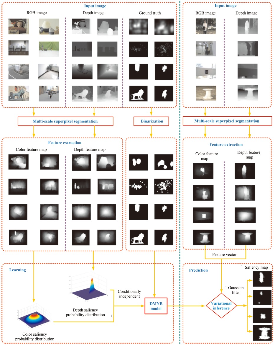
Fig. 1 The flowchart of the proposed model. The framework of our model consists of two stages: the training stage shown in the left part of the figure and the testing stage shown in the right part of the figure. In this work, we perform experiments based on the EyMIR dataset in [32], NUS dataset in [11], NLPR dataset in [29] and NJU-DS400 dataset in [31].
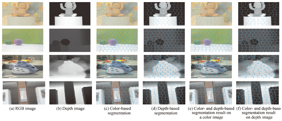
Fig. 2 Visual samples for superpixel segmentation of RGB-D images with $\mathcal{S}=40$. Rows 1-4: comparative results on the EyMIR dataset, NUS dataset, NLPR dataset and NJU-DS400 dataset, respectively.

Fig. 3 Visual illustration for the saliency measure based on manifold ranking, where patches from corners of images marked as red is defined as pseudo-background.
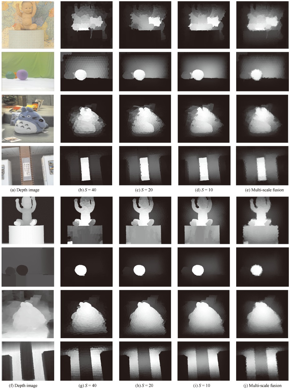
Fig. 4 Visual samples of different color and depth feature maps. Rows 1−4: color feature maps of the EyMIR dataset, NUS dataset, NLPR dataset and NJU-DS400 dataset, respectively. Rows 5−8: depth feature maps of the EyMIR dataset, NUS dataset, NLPR dataset and NJU-DS400 dataset, respectively.
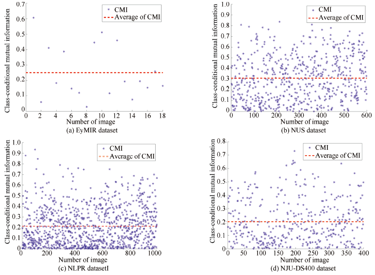
Fig. 5 Visual results for class-conditional mutual information between color-based contrast features and depth-based contrast features on four RGB-D image datasets.

Fig. 6 Graphical models of DMNB for saliency estimation. $\pmb{y}$ and $\pmb{x}$ are the corresponding observed states, and $\pmb{z}$ is the hidden variable.
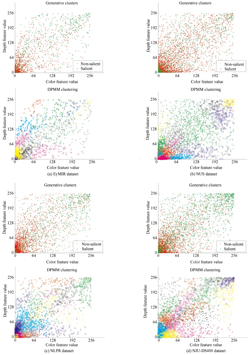
Fig. 7 Visual result for the number of components $K$ in the DMNB model: generative clusters vs DPMM clustering. Row 1: generative clusters for four RGB-D image datasets, where green and red denote distribution of salient and non-salient features, respectively. Row 2: DPMM clustering for four RGB-D image datasets, where the number of colors and shapes of the points denote the number of components $K$. The appropriate number of mixture components to use in DMNB model for saliency estimation is generally unknown, and DPMM provides an attractive alternative to current method. We find $K=26$, $34$, $28$, and $32$ using DPMM on the EyMIR dataset, NUS dataset, NLPR dataset and NJU-DS400 dataset, respectively.
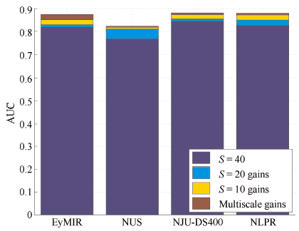
Fig. 8 The effects of the number of scales $\mathcal{S}$ on the EyMIR, NUS, NLPR and NJU-DS400 datasets. A single scale produces inferior results.
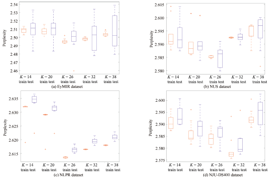
Fig. 9 The perplexity for different $K$ components in the DMNB model in terms of the four datasets. We use 10-fold cross-validation with the parameter $K$ for DMNB models. The $K$ found using DPMM was adjusted over a wide range in a 10-fold cross-validation.
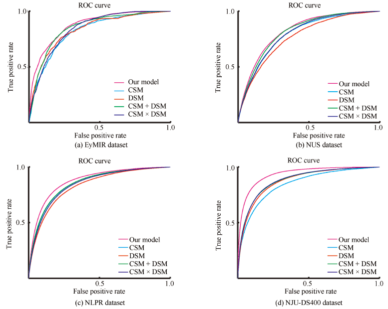
Fig. 10 The ROC curves of different feature map and their linear fusions. $+$ indicates a linear combination strategy, and $\times$ indicates a weighting method based on multiplication.
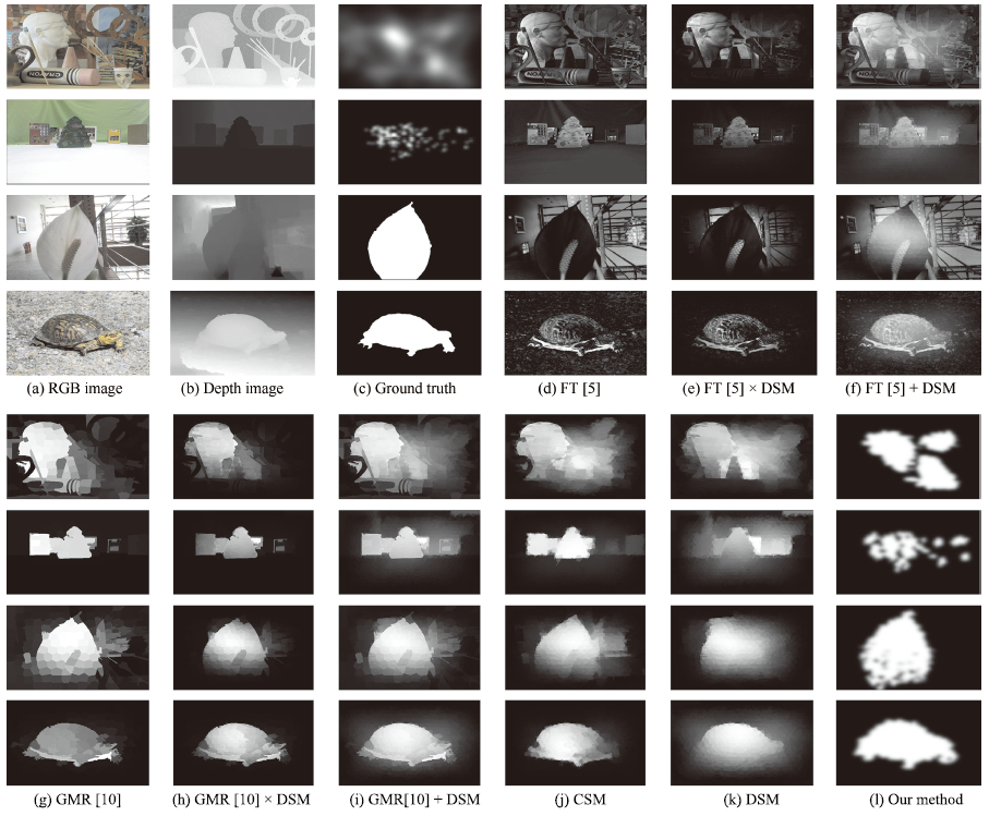
Fig. 11 Visual comparison of the saliency estimations of the different 2D methods with DSM. $+$ indicates a linear combination strategy, and $\times$ indicates a weighting method based on multiplication. DSM means depth saliency map, which is produced by our proposed depth feature map. CSM means color saliency map, which is produced by our proposed color feature map.
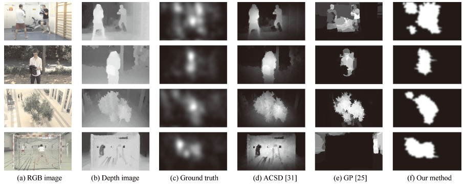
Fig. 12 Visual comparison of saliency estimations of different 3D methods based on the EyMIR dataset.
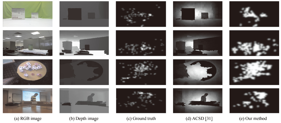
Fig. 13 Visual comparison of saliency estimations of different 3D methods based on the NUS dataset.
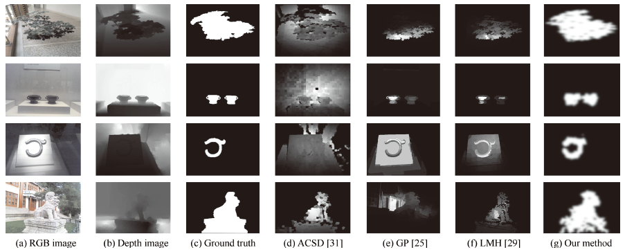
Fig. 14 Visual comparison of saliency estimations of different 3D methods based on the NLPR dataset.
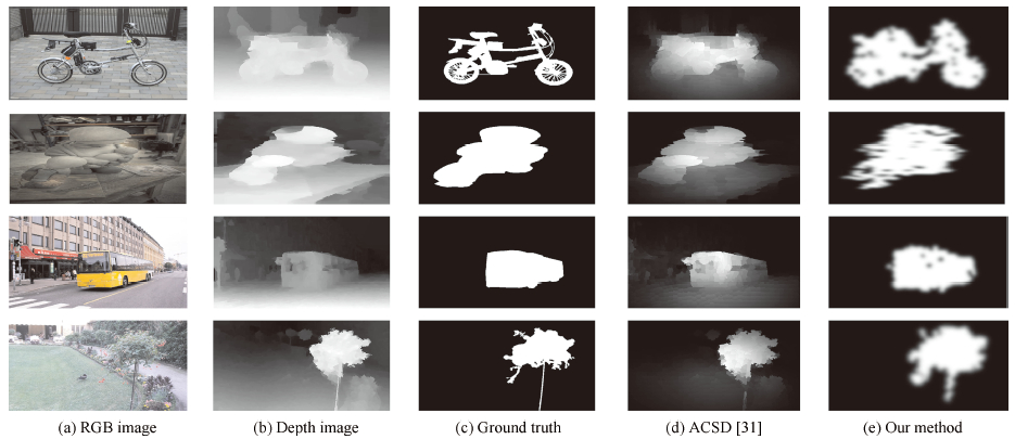
Fig. 15 Visual comparison of the saliency estimations of different 3D methods based on the NJU-DS400 dataset.
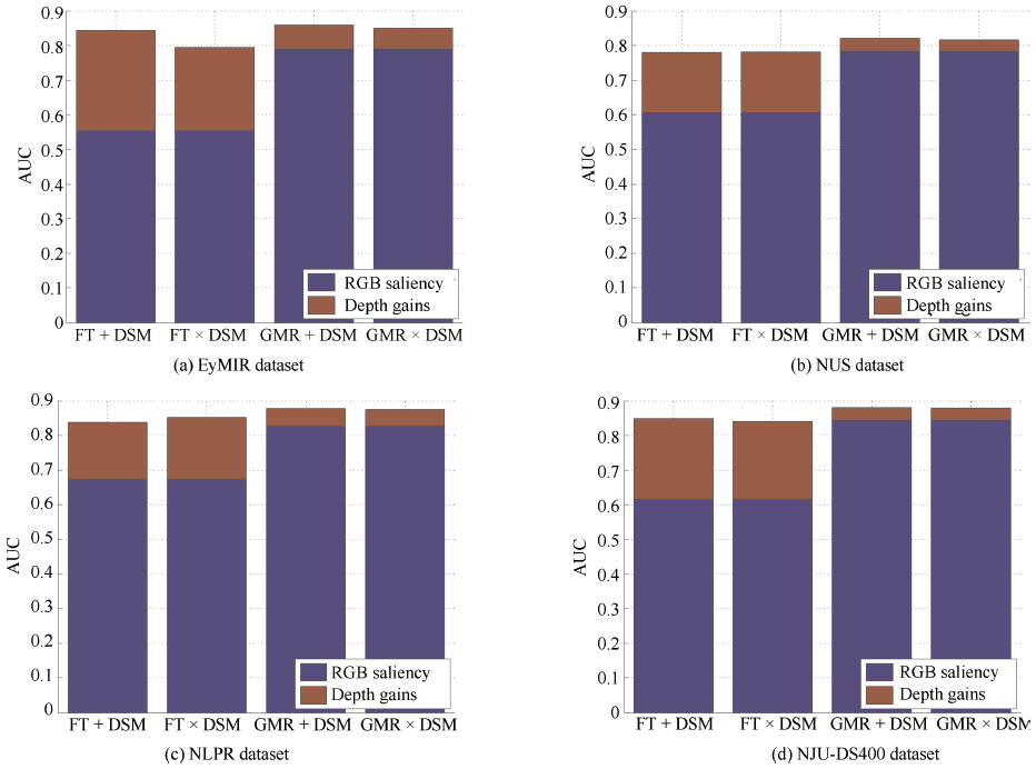
Fig. 16 The quantitative comparisons of the performance of the depth cues. + indicates a linear combination strategy, and indicates a weighting method based on multiplication.
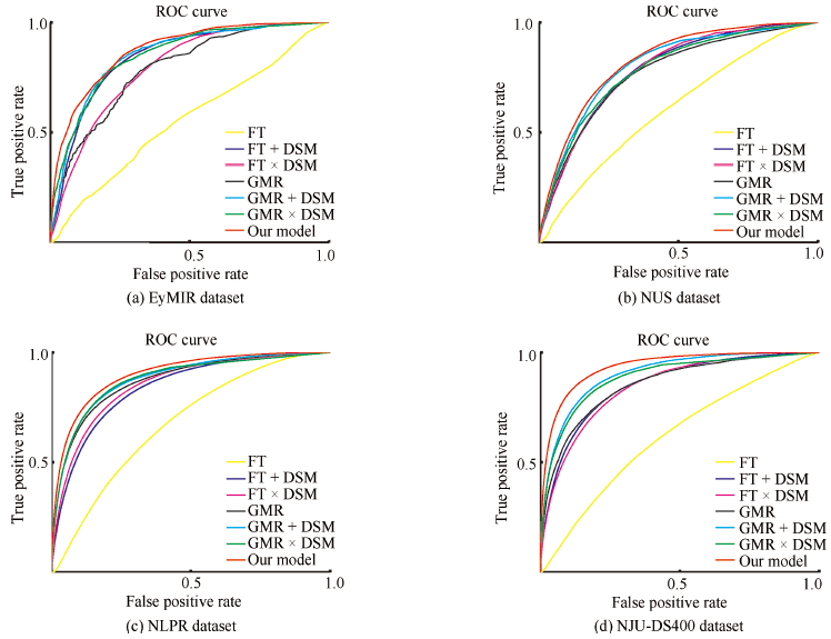
Fig. 17 The quantitative comparisons of the performances of depth cues. + indicates a linear combination strategy, and indicates a weighting method based on multiplication.

Fig. 18 The ROC curves of different 3D saliency detection models in terms of the EyMIR dataset, NUS dataset, NLPR dataset and NJU-DS400.

Fig. 19 The F-measures of different 3D saliency detection models when used on the EyMIR dataset, NUS dataset, NLPR dataset and NJU-DS400.
Algorithm 1. Superpixel segmentation of the RGB-D images Input: $m$, $\mathcal{S}$, $\omega_d$ and $IterNum$.
Initialization: Initialize clusters $C_i=[l_i, a_i, b_i, d_i, x_i, y_i]^T$ by sampling pixels at regular grid steps $\mathcal{S}$ by computing the average $labdxy$ vector, where $[l_i, a_i, b_i]$ is the $L, a, b$ values of the CIELAB color space and $[x_i, y_i]$ is the pixel coordinates of $i$th grid in the RGB-D image pair.
Set label $l(p)=-1$ and distance $d(p)=\infty$ for each pixel $p.$
Output: $d(p)$.
1: Perturb cluster centres in a $3\times 3$ neighbourhood to the lowest gradient position in the RGB image.
2: for $IterNum$ do
3: for each cluster centre $C_i$ do
4: Assign the best matching pixels from a $2\mathcal{S}\times2\mathcal{S}$ square neighbourhood around the cluster centre according to the distance measure $D_s$ in (1).
for each pixel p in a $2\mathcal{S}\times2\mathcal{S}$ region around $C_i$ do
Compute the distance $D_s$ between $C_i$ and $labdxy_p$
if $D_s < d(p) $ then
Set $d(p) = D_s$
Set $l(p) = i $
end if
end for
5: end for
6: Computer new cluster centres. After all the pixels are associated with the nearest cluster center, a new center is computed as the average $labdxy$ vector of all the pixels belonging to the cluster.
7: end for
8: Enforce connectivity. 下载: 导出CSV
Algorithm 2. Generative process for saliency detection following the DMNB model 1: Input: $\alpha$, $\eta$.
2: Choose a component proportion: $\theta\sim p(\theta|\alpha)$.
3: For each feature:
choose a component $\pmb{z}_j \sim p({\pmb z}_j|\theta)$;
choose a feature value ${\pmb x}_j\sim p({\pmb x}_j|\pmb{z}_j, \Omega_j)$.
4: Choose the label: ${\pmb y} \sim p({\pmb y}| {\pmb z}_j, \eta)$.
下载: 导出CSV
Algorithm 3. Variational EM algorithm for DMNB 1: repeat
2: E-step: Given $(\alpha^{m-1}, \Omega^{m-1}, \eta^{m-1})$, for each feature value and label, find the optimal variational parameters
$(\gamma_i^{m}, \phi_i^{m}, \xi_i^{m})=$ $\arg\max\mathcal{L}(\gamma_i, \phi_i, \xi_i;\alpha^{m-1}, \Omega^{m-1}, \eta^{m-1})$.
Then, $\mathcal{L}(\gamma_i^{m}, \phi_i^{m}, \xi_i^{m};\alpha, \Omega, \eta)$ gives a lower bound to $\log p(\pmb{y}_i, \pmb{x}_{1:N}|\alpha, \Omega, \eta)$.
3: M-step: Improved estimates of the model parameters $(\alpha, \Omega, \eta)$ are obtained by maximizing the aggregate lower bound:
$(\alpha^{m}, \Omega^{m}, \eta^{m})= \arg\max_{(\alpha, \Omega, \eta)} \sum_{i=1}^N \mathcal{L}(\gamma_i^{m}, \phi_i^{m}, \xi_i^{m}; \alpha, \Omega, \eta)$.
4: until $\sum_{i=1}^N\mathcal{L} (\gamma_i^{m}, \phi_i^{m}, \xi_i^{m};\alpha^{m}, \Omega^{m}, \eta^{m})$
$-\sum_{i=1}^N\mathcal{L} (\gamma_i^{m+1}, \phi_i^{m+1}, \xi_i^{m+1};\alpha^{m+1}, \Omega^{m+1}, \eta^{m+1})$
$\leq$ threshold.
下载: 导出CSV
Table Ⅰ Summary of Parameters
Name Range Description $m$ [1, 40] the weight of spatial proximity $\mathcal{S}$ $> 8$ the grid interval $m_d$ (0, 1] the weight of depth distance $IterNum$ [10, 200] the iteration number of superpixel segmentation $L$ [2, 10] the level of multi-sacle superpixel segmentation $\omega_c^l$ (0, 1) the weight of color feature map at $l$ scale $\omega_d^l$ (0, 1) the weight of depth feature map at $l$ scale $\tau$ (0, 1) a CMI threshold $\alpha$ (0, 40] the parameter of a Dirichlet distribution $\theta$ (0, 1) the parameter of a Multinomial distribution $\eta$ ($-$2.0, 2.0) the parameter of a Bernoulli distribution $\Omega$ ((0, 255), (1, $10^3$)) the parameter of a Gaussian distribution $K$ $> 2$ the number of components of DMNB
下载: 导出CSV
-
[1] P. Le Callet and E. Niebur, "Visual attention and applications in multimedia technologies, " Proc. IEEE, vol. 101, no. 9, pp. 2058-2067, Sep. 2013. doi: 10.1109/JPROC.2013.2265801 [2] A. Borji and L. Itti, "State-of-the-art in visual attention modeling, " IEEE Trans. Pattern Anal. Mach. Intell., vol. 35, no. 1, pp. 185-207, Jan. 2013. doi: 10.1109/TPAMI.2012.89 [3] A. Borji, D. N. Sihite, and L. Itti, "Salient object detection: A benchmark, " in Proc. 12th European Conf. Computer Vision, Florence, Italy, 2012, pp. 414-429. [4] L. Itti, C. Koch, and E. Niebur, "A model of saliency-based visual attention for rapid scene analysis, " IEEE Trans. Pattern Anal. Mach. Intell., vol. 20, no. 11, pp. 1254-1259, Nov. 1998. doi: 10.1109/34.730558 [5] R. Achanta, S. Hemami, F. Estrada, and S. Susstrunk, "Frequency-tuned salient region detection, " in Proc. 2009 IEEE Conf. Computer Vision and Pattern Recognition, Miami, FL, USA, 2009, pp. 1597-1604. [6] X. D. Hou and L. Q. Zhang, "Saliency detection: A spectral residual approach, " in Proc. 2007 IEEE Conf. Computer Vision and Pattern Recognition, Minneapolis, MN, USA, 2007, pp. 1-8. [7] J. Harel, C. Koch, and P. Perona, "Graph-based visual saliency, " in Advances in Neural Information Processing Systems, Vancouver, British Columbia, Canada, 2006, pp. 545-552. [8] M. M. Cheng, G. X. Zhang, N. J. Mitra, X. L. Huang, and S. M. Hu, "Global contrast based salient region detection, " in Proc. 2011 IEEE Conf. Computer Vision and Pattern Recognition, Providence, RI, USA, 2011, pp. 409-416. [9] S. Goferman, L. Zelnik-Manor, and A. Tal, "Context-aware saliency detection, " in Proc. 2010 IEEE Conf. Computer Vision and Pattern Recognition, San Francisco, CA, USA, 2010, pp. 2376-2383. [10] C. Yang, L. H. Zhang, H. C. Lu, X. Ruan, and M. H. Yang, "Saliency detection via graph-based manifold ranking, " in Proc. 2013 IEEE Conf. Computer Vision and Pattern Recognition, Portland, OR, USA, 2013, pp. 3166-3173. [11] C. Y. Lang, T. V. Nguyen, H. Katti, K. Yadati, M. Kankanhalli, and S. C. Yan, "Depth matters: Influence of depth cues on visual saliency, " in Proc. 12th European Conf. Computer Vision, Florence, Italy, 2012, pp. 101-115. [12] K. Desingh, K. M. Krishna, D. Rajan, and C. V. Jawahar, "Depth really matters: Improving visual salient region detection with depth, " in Proc. 2013 British Machine Vision Conf. , Bristol, England, 2013, pp. 98. 1-98. 11. [13] J. L. Wang, Y. M. Fang, M. Narwaria, W. S. Lin, and P. Le Callet, "Stereoscopic image retargeting based on 3D saliency detection, " in Proc. 2014 IEEE Int. Conf. Acoustics, Speech and Signal Processing, Florence, Italy, 2014, pp. 669-673. [14] H. Kim, S. Lee, and A. C. Bovik, "Saliency prediction on stereoscopic videos, " IEEE Trans. Image Process., vol. 23, no. 4, pp. 1476-1490, Apr. 2014. doi: 10.1109/TIP.2014.2303640 [15] Y. Zhang, G. Y. Jiang, M. Yu, and K. Chen, "Stereoscopic visual attention model for 3D video, " in Proc. 16th Int. Multimedia Modeling Conf. , Chongqing, China, 2010, pp. 314-324. [16] M. Uherčík, J. Kybic, Y. Zhao, C. Cachard, and H. Liebgott, "Line filtering for surgical tool localization in 3D ultrasound images, " Comput. Biol. Med., vol. 43, no. 12, pp. 2036-2045, Dec. 2013. doi: 10.1016/j.compbiomed.2013.09.020 [17] Y. Zhao, C. Cachard, and H. Liebgott, "Automatic needle detection and tracking in 3D ultrasound using an ROI-based RANSAC and Kalman method, " Ultrason. Imaging, vol. 35, no. 4, pp. 283-306, Oct. 2013. doi: 10.1177/0161734613502004 [18] Y. M. Fang, J. L. Wang, M. Narwaria, P. Le Callet, and W. S. Lin, "Saliency detection for stereoscopic images, " IEEE Trans. Image Process., vol. 23, no. 6, pp. 2625-2636, Jun. 2014. doi: 10.1109/TIP.2014.2305100 [19] A. Ciptadi, T. Hermans, and J. M. Rehg, "An in depth view of saliency, " in Proc. 2013 British Machine Vision Conf. , Bristol, England, 2013, pp. 9-13. [20] P. L. Wu, L. L. Duan, and L. F. Kong, "RGB-D salient object detection via feature fusion and multi-scale enhancement, " in Proc. 2015 Chinese Conf. Computer Vision, Xi'an, China, 2015, pp. 359-368. [21] F. F. Chen, C. Y. Lang, S. H. Feng, and Z. H. Song, "Depth information fused salient object detection, " in Proc. 2014 Int. Conf. Internet Multimedia Computing and Service, Xiamen, China, 2014, pp. 66. [22] I. Iatsun, M. C. Larabi, and C. Fernandez-Maloigne, "Using monocular depth cues for modeling stereoscopic 3D saliency, " in Proc. 2014 IEEE Int. Conf. Acoustics, Speech and Signal Processing, Florence, Italy, 2014, pp. 589-593. [23] N. Ouerhani and H. Hugli, "Computing visual attention from scene depth, " in Proc. 15th Int. Conf. Pattern Recognition, Barcelona, Spain, 2000, pp. 375-378. [24] H. Y. Xue, Y. Gu, Y. J. Li, and J. Yang, "RGB-D saliency detection via mutual guided manifold ranking, " in Proc. 2015 IEEE Int. Conf. Image Processing, Quebec City, QC, Canada, 2015, pp. 666-670. [25] J. Q. Ren, X. J. Gong, L. Yu, W. H. Zhou, and M. Y. Yang, "Exploiting global priors for RGB-D saliency detection, " in Proc. 2015 IEEE Conf. Computer Vision and Pattern Recognition Workshops, Boston, MA, USA, 2015, pp. 25-32. [26] H. K. Song, Z. Liu, H. Du, G. L. Sun, and C. Bai, "Saliency detection for RGBD images, " in Proc. 7th Int. Conf. Internet Multimedia Computing and Service, Zhangjiajie, Hunan, China, 2015, pp. Atricle ID 72. [27] J. F. Guo, T. W. Ren, J. Bei, and Y. J. Zhu, "Salient object detection in RGB-D image based on saliency fusion and propagation, " in Proc. 7th Int. Conf. Internet Multimedia Computing and Service, Zhangjiajie, Hunan, China, 2015, pp. Atricle ID 59. [28] X. X. Fan, Z. Liu, and G. L. Gun, "Salient region detection for stereoscopic images, " in Proc. 19th Int. Conf. Digital Signal Processing, Hong Kong, China, 2014, pp. 454-458. [29] H. W. Peng, B. Li, W. H. Xiong, W. M. Hu, and R. R. Ji, "Rgbd salient object detection: A benchmark and algorithms, " in Proc. 13th European Conf. Computer Vision, Zurich, Switzerland, 2014, pp. 92-109. [30] Y. Z. Niu, Y. J. Geng, X. Q. Li, and F. Liu, "Leveraging stereopsis for saliency analysis, " in Proc. 2012 IEEE Conf. Computer Vision and Pattern Recognition, Providence, RI, USA, 2012, pp. 454-461. [31] R. Ju, L. Ge, W. J. Geng, T. W. Ren, and G. S. Wu, "Depth saliency based on anisotropic center-surround difference, " in Proc. 2014 IEEE Int. Conf. Image Processing, Paris, France, 2014, pp. 1115-1119. [32] J. L. Wang, M. P. Da Silva, P. Le Callet, and V. Ricordel, "Computational model of stereoscopic 3D visual saliency, " IEEE Trans. Image Process., vol. 22, no. 6, pp. 2151-2165, Jun. 2013. doi: 10.1109/TIP.2013.2246176 [33] I. Iatsun, M. C. Larabi, and C. Fernandez-Maloigne, "Visual attention modeling for 3D video using neural networks, " in Proc. 2014 Int. Conf. 3D Imaging, Liege, Belgium, 2014, pp. 1-8. [34] Y. M. Fang, W. S. Lin, Z. J. Fang, P. Le Callet, and F. N. Yuan, "Learning visual saliency for stereoscopic images, " in Proc. 2014 IEEE Int. Conf. Multimedia and Expo Workshops, Chengdu, China, 2014, pp. 1-6. [35] L. Zhu, Z. G. Cao, Z. W. Fang, Y. Xiao, J. Wu, H. P. Deng, and J. Liu, "Selective features for RGB-D saliency, " in Proc. 2015 Conf. Chinese Automation Congr. , Wuhan, China, 2015, pp. 512-517. [36] G. Bertasius, H. S. Park, and J. B. Shi, "Exploiting egocentric object prior for 3D saliency detection, " arXiv preprint arXiv: 1511. 02682, 2015. [37] H. H. Shan, A. Banerjee, and N. C. Oza, "Discriminative mixed-membership models, " in Proc. 2009 IEEE Int. Conf. Data Mining, Miami, FL, USA, 2009, pp. 466-475. [38] R. Achanta, A. Shaji, K. Smith, A. Lucchi, P. Fua, and S. Süsstrunk, "SLIC superpixels compared to state-of-the-art superpixel methods, " IEEE Trans. Pattern Anal. Mach. Intell., vol. 34, no. 11, pp. 2274-2282, Nov. 2012. doi: 10.1109/TPAMI.2012.120 [39] I. Rish, "An empirical study of the naive Bayes classifier, " J. Univ. Comput. Sci., vol. 3, no. 22, pp. 41-46, Aug. 2001. [40] D. M. Blei and M. I. Jordan, "Variational inference for Dirichlet process mixtures, " Bayes. Anal., vol. 1, no. 1, pp. 121-143, Mar. 2006. doi: 10.1214/06-BA104 -

 下载:
下载:

计量
- 文章访问数: 2562
- HTML全文浏览量: 296
- PDF下载量: 1043
- 被引次数: 0
