

A Robust Minimum Volume Based Algorithm with Automatically Estimating Regularization Parameters for Hyperspectral Unmixing
-
摘要: 对高光谱图像解混的目的在于从低空间分辨率的高光谱图像中找到端元与对应的丰度.本文根据解混算法中的最小体积准则,提出了一种自适应鲁棒最小体积高光谱解混算法(Robust minimum volume based algorithm with automatically estimating regularization parameters for hyperspectral unmixing,RMVHU).本算法通过引入负数惩罚正则项,替换了同类算法中的丰度非负性约束(Non-negativity constraint,ANC),使算法对图像中的噪声与异常值具有更强的鲁棒性;采用循环最小化方法,将非凸优化问题分解为凸优化子问题,然后应用交替方向乘子法解决随着像素点个数增大带来的求解困难问题;对于正则项系数,本算法提出了一种自适应调整策略,提高了算法的收敛性,并且通过定性分析,说明了该调整方法的合理性.将算法应用于合成数据与实际数据,实验结果表明,与同类算法相比,本文提出的算法能够取得更为优秀的效果.Abstract: Hyperspectral unmixing aims at finding hidden endmembers and their corresponding abundances from hyperspectral images with low spatial resolution. Based on the well-known minimum volume (MV) rule in geometrical based approaches, a robust minimum volume based algorithm with automatically estimating regularization parameters for hyperspectral unmixing (RMVHU) is proposed. In this algorithm, the ANC constraint is replaced with a negative number punished regularizer which may lead to a more robust result to outliers and noise. A cyclic minimization algorithm is used to split the nonconvex RMVHU problem into convex subproblems, and ADMM is referred to sovle the large scale optimization problem with the increasing number of pixels in the image. To improve the convergence of the algorithm, a strategy to estimate the regularization parameters of the regularizer automatically is proposed. Compared with some existing geometrical based methods, experimental results show the superiority of the RMVHU algorithm on both synthetic datasets and real datasets.1) 本文责任编委 胡清华
-
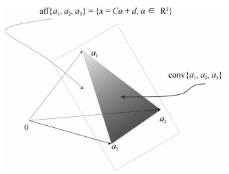
图 1 顶点个数为3时, 凸包与仿射集的概念说明
Fig. 1 Illustration of convex hull and affine hull when the number of vertices is three
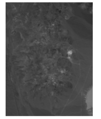
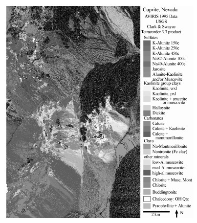
图 3 Cuprite地区高光谱图像伪彩色子图, R: 2.109 ${\rm \mu m}$, G: 2.209 ${\rm \mu m}$, B: 2.308 ${\rm \mu m}$
Fig. 3 The Pseudo color subimage of the AVIRIS Cuprite dataset, R: 2.109 ${\rm \mu m}$, G: 2.209 ${\rm \mu m}$, B: 2.308 ${\rm \mu m}$
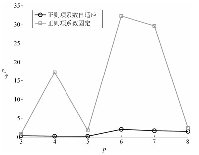
图 7 正则项系数固定或自适应变化时, 各算法平均光谱角距离
Fig. 7 The average spectral angle distance of different algorithms when the regularization parameter is fixed or changes automatically

图 8 正则项系数固定或自适应变化时, 各算法平均均方根误差
Fig. 8 The average root mean square error of different algorithms when the regularization parameter is fixed or changes automatically
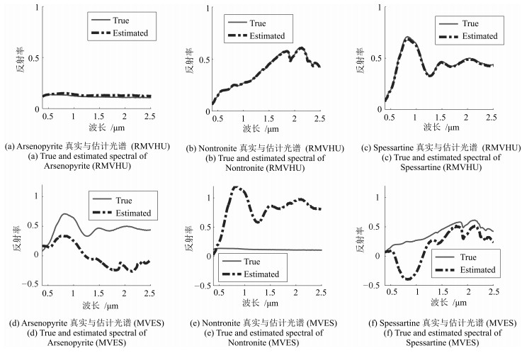
图 9 RMVHU与MVES端元估计结果, (a)、(b)、(c)为RMVHU的端元估计结果, (d)、(e)、(f)为MVES的端元估计结果
Fig. 9 Estimated results of endmembers via two algorithms: RMVHU and MVES ((a)、(b)、(c) are the results of RMVHU and (d)、(e)、(f) are the results of MVES)
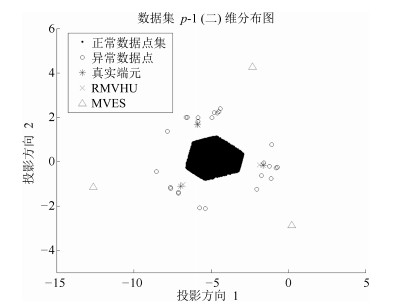
图 10 数据集与端元在$p-1$ (二)维子空间的投影
Fig. 10 Two dimensional subspace projection of datasets, estimated endmembers and real endmembers
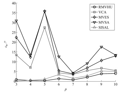
图 11 端元个数变化时, 各算法平均光谱角距离
Fig. 11 The average spectral angle distance of different algorithms when the number of endmembers changes
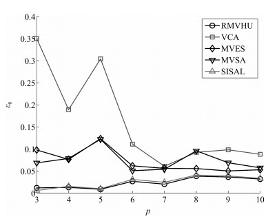
图 12 端元个数变化时, 各算法平均均方根误差
Fig. 12 The average root mean square error of different algorithms when the number of endmembers changes
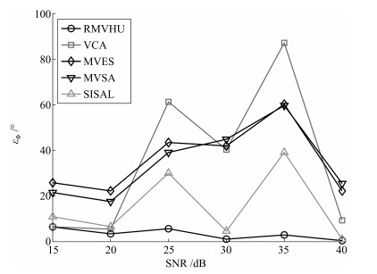
图 13 在不同噪声大小下, 各算法平均光谱角距离
Fig. 13 The average spectral angle distance of different algorithms when SNR changes
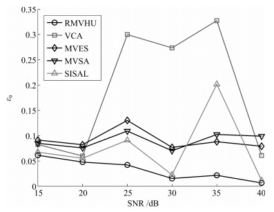
图 14 在不同噪声大小下, 各算法平均均方根误差
Fig. 14 The average root mean square error of different algorithms when SNR changes
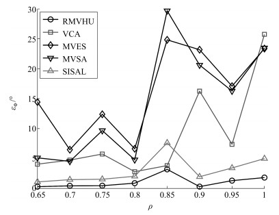
图 15 在不同混合度下, 各算法平均光谱角距离
Fig. 15 The average spectral angle distance of different algorithms when the purity of pixels changes
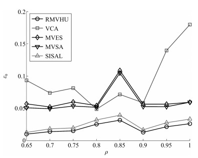
图 16 在不同混合度下, 各算法平均均方根误差
Fig. 16 The average root mean square error of different algorithms when the purity of pixels changes
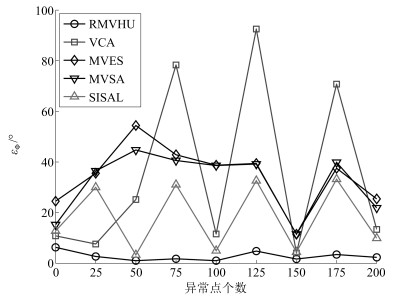
图 17 在不同异常点个数下, 各算法平均光谱角距离
Fig. 17 The average spectral angle distance of different algorithms when the number of outliers changes
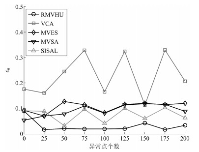
图 18 在不同异常点个数下, 各算法平均均方根误差
Fig. 18 The average root mean square error of different algorithms when the number of outliers changes

图 19 在不同像素点个数下, 各算法平均光谱角距离
Fig. 19 The average spectral angle distance of different algorithms when the number of pixels changes
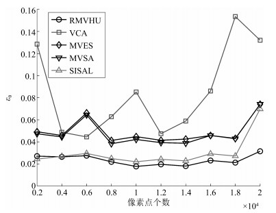
图 20 在不同像素点个数下, 各算法平均均方根误差
Fig. 20 The average root mean square error of different algorithms when the number of pixels changes
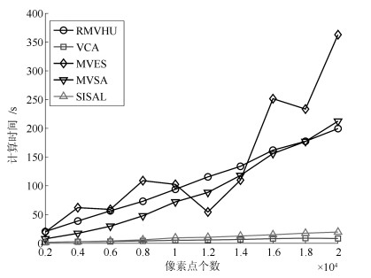
图 21 在不同像素点个数下, 各算法运行时间
Fig. 21 Computational time of different algorithms when the number of pixels changes
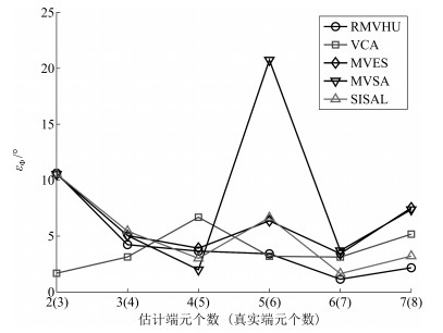
图 22 在错估端元个数时, 各算法平均光谱角距离
Fig. 22 The average spectral angle distance of different algorithms when the number of endmembers is incorrectly estimated
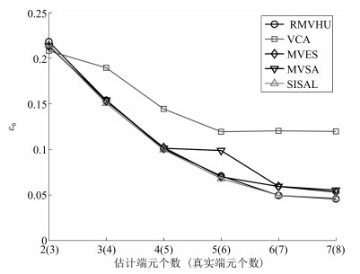
图 23 在错估端元个数时, 各算法平均均方根误差
Fig. 23 The average root mean square error of different algorithms when the number of endmembers is incorrectly estimated
表 1 数学符号及其意义
Table 1 Mathematical notations and their meaning
符号 符号意义 ${\bf R}$ 实数 ${\bf R}^{{L}}$ ${L}$维向量 ${\bf R}^{{L}\times {\rm N}}$ ${L}\times {\rm N}$维矩阵 ${\bf R}_{+}$ 非负实数 ${\bf R}_+^{L}$ 非负${L}$维向量 ${\bf R}_{+}^{{L}\times {N}}$ 非负${L}\times {N}$维矩阵 $1_{N}$ ${N}\times 1$维全1列向量 $I_{N}$ ${N}\times {N}$维单位矩阵 $X^†$ $X$的广义逆矩阵 $\boldsymbol{ e}_i$ 第$i$个元素为1, 其他元素为0的单位列向量 $\boldsymbol{x}\succeq {a}, {\boldsymbol{x}}\in {\bf R}^{{L}}$ $L$维列向量$\boldsymbol{x}$中所有元素均不小于$a$ $l_{\bf R_{+}}(\boldsymbol{x})$ $l_{\bf R_{+}}(\boldsymbol{x})=\begin{cases} 0, &\boldsymbol{x}\succeq 0 \\ + \infty, & \mbox{其他} \end{cases}$ ${\rm sgn} (y)$ ${\rm sgn}(y)=\begin{cases} 1, &y > 0 \\ 0, & y=0\\-1, &y < 0 \end{cases}$  下载: 导出CSV
表 2 RMVHU中求解子问题$p^{*}$的算法步骤
Table 2 Steps for solving subproblem $p^{*}$ in RMVHU
算法名称: 求解问题$p^{*}$的ADMM算法步骤 步骤1: 设初值$k=0, \mu > 0, \boldsymbol{ x}_0, {z}_1^0, {d}_1^0, \boldsymbol{ z}_2^0, \boldsymbol{ d}_2^0 $ 步骤2: 更新$\boldsymbol{x}$: $\boldsymbol{ x}^{k+1} = \arg\; \mathop {\min }\limits_\boldsymbol{ x}L(\boldsymbol{ x}, {z_1^k}, \boldsymbol{ z}_2^k, d_1^k, \boldsymbol{ d}_2^k) $ 步骤3: 更新$z_1$: ${z_1^{k+1} }= \arg\; \underset{z_1}{\min}L(\boldsymbol{ x}^{k+1}, {z_1}, \boldsymbol{ z}_2^k, d_1^k, \boldsymbol{ d}_2^k) $ 步骤4: 更新$\boldsymbol{ z}_2$: $\boldsymbol{ z}_2^{k+1} = \arg\; \underset{\boldsymbol{ z}_2}{\min}L(\boldsymbol{ x}^{k+1}, {z_1^{k+1}}, \boldsymbol{ z}_2, d_1^k, \boldsymbol{ d}_2^k) $ 步骤5: 更新$d_1$: ${d_1^{k+1} }= d_1^k -(\boldsymbol{ c}^{\rm T} \boldsymbol{ x}^{k+1} -z_1^{k+1})$ 步骤6: 更新$\boldsymbol{ d}_2$: $\boldsymbol{ d}_2^{k+1} = \boldsymbol{ d}_2^{k} -(A \boldsymbol{ x}^{k+1} +\boldsymbol{ b} -\boldsymbol{ z}_2^{k+1})$ 步骤7: 判断是否满足迭代停止条件, 若满足, 则转步骤8, 否则$k=k+1$, 转步骤2. 步骤8: 输出$\boldsymbol{ x}^{k+1}$:
下载: 导出CSV
表 3 RMVHU算法步骤
Table 3 Procedure for solving RMVHU
算法名称: RMVHU 输入: 端元个数$\ p$, 高光谱图像数据集$Y\in{\bf R}^{ {\ L} \times {\ N}}$, 收敛阈值$\varepsilon$, 最大迭代步数值$\ M$. 输出: 端元矩阵$A$, 丰度矩阵$S$. 步骤1: 根据式(14)与(16)对数据集$Y$进行降维, 得到降维后的光谱数据集$\tilde{Y}\in{\bf R}^{ ({\ p} -1) \times {\ N}}$. 步骤2: 设置当前迭代步数$i=0$, 并寻找满足如下条件的矩阵$H$与$\ g$作为初始迭代值: $ {H} \tilde{\boldsymbol{ y}}[n] -\boldsymbol{ g} \succeq 0, 1_{ {\ p} -1}^{\rm T}({H} \tilde{\boldsymbol{ y}}[n] -\boldsymbol{ g})\leq 1, \forall n=1, \cdots, {\ N} $} 步骤3: 对$k=1, 2, \cdots, {\ p}-1$, 执行步骤4与步骤5. 步骤4: 使用表 2中的ADMM算法与式(51)自适应更新, 求解子问题(28)与(29), 得到单步最优解$(\boldsymbol{ h}_{k}^{-}, g_{k}^{-})$与$(\boldsymbol{ h}_{k}^{+}, g_{k}^{+})$及其对应的目标函数值$p^*$与$q^*$. 步骤5: 如果$p^* < q^*$, 则$(\boldsymbol{ h}_{k}, g_{k}) = (\boldsymbol{ h}_{k}^{-}, g_{k}^{-})$, 否则$(\boldsymbol{ h}_{k}, g_{k}) = (\boldsymbol{ h}_{k}^{+}, g_{k}^{+})$, 更新矩阵$H$与$\boldsymbol{ g}$相应的元素得到$H^*$与$\boldsymbol{ g}^*$. 步骤6: 如果$\left| {\left| {\det \left({{H^*}} \right)} \right| -\rho }\right|/\rho < \varepsilon$, 或者$i > {\ M}$, 则转步骤7, 否则$i=i+1$, $\rho = {\det \left({{H^*}} \right)}$, 应用式(50)更新正则系数$\lambda $, 转步骤3. 步骤7: 根据式(48)、(49)得到端元矩阵$A$与丰度矩阵$S$.
下载: 导出CSV
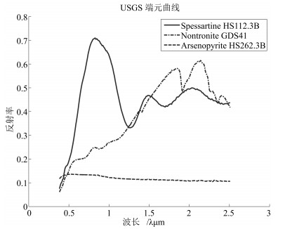
表 4 RMVHU与MVES算法的光谱角距离与平均光谱角距离
Table 4 Spectral angle distance and average spectral angle distance via RMVHU and MVES
端元名称 RMVHU MVES Spessartine 0.30 1.86 Nontronite 0.26 18.29 Arsenopyrite 2.03 120.60 $\varepsilon_\theta$ (°) 0.87 46.92
下载: 导出CSV
表 5 RMVHU与MVES算法的均方根误差与平均均方根误差
Table 5 Root mean square error and average root mean square error via RMVHU and MVES
端元名称 RMVHU MVES Spessartine 0.012 0.239 Nontronite 0.008 0.151 Arsenopyrite 0.013 0.165 $\varepsilon_\theta$ (°) 0.011 0.185
下载: 导出CSV
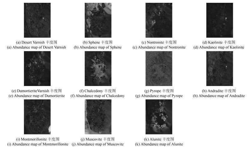
表 6 RMVHU、VCA、MVES、MVSA、SISAL算法提取端元与真实端元的光谱角距离
Table 6 The spectral angle distance of real datasets via unmixing algorithms: RMVHU, VCA, MVES, MVSA and SISAL
物质 RMVHU VCA MVES MVSA SIS (a) Desert Varnish 15.08 21.48 16.86 16.02 22.35 (b) Sphene 86.03 28.07 62.25 59.24 18.33 (c) Nontronite 33.57 18.22 35.51 33.13 33.80 (d) Kaolinite 20.32 31.95 29.44 37.59 14.90 (e) Dumortierite 14.55 24.94 23.75 21.60 64.74 (f) Chalcedony 15.15 16.26 38.04 39.76 28.07 (g) Pyrope 23.74 29.89 44.67 54.42 63.03 (h) Andradite 17.18 32.38 45.62 60.30 27.50 (i) Montmorillonite 21.24 46.39 35.85 41.08 21.20 (j) Muscovite 20.66 37.47 65.06 78.46 24.64 (k) Alunite 15.72 37.55 38.57 29.36 12.03 ${\varepsilon_\phi}$ (°) 25.75 29.51 39.60 42.81 30.05
下载: 导出CSV
-
[1] 潘宗序, 禹晶, 肖创柏, 孙卫东.基于光谱相似性的高光谱图像超分辨率算法.自动化学报, 2014, 40(12):2797-2807 http://www.aas.net.cn/CN/abstract/abstract18558.shtmlPan Zong-Xu, Yu Jing, Xiao Chuang-Bai, Sun Wei-Dong. Spectral similarity-based super resolution for hyperspectral images. Acta Automatica Sinica, 2014, 40 (12):2797-2807 http://www.aas.net.cn/CN/abstract/abstract18558.shtml [2] 倪鼎, 马洪兵.基于近邻协同的高光谱图像谱-空联合分类.自动化学报, 2015, 41 (2):273-284 http://www.aas.net.cn/CN/abstract/abstract18606.shtmlNi Ding, Ma Hong-Bing. Spectral-spatial classification of hyperspectral images based on neighborhood collaboration. Acta Automatica Sinica, 2015, 41 (2):273-284 http://www.aas.net.cn/CN/abstract/abstract18606.shtml [3] Du B, Zhang L P. A discriminative metric learning based anomaly detection method. IEEE Transactions on Geoscience and Remote Sensing, 2014, 52 (11):6844-6857 doi: 10.1109/TGRS.2014.2303895 [4] Lin C H, Chi C Y, Wang Y H, Chan T H. A fast hyperplane-based minimum-volume enclosing simplex algorithm for blind hyperspectralunmixing. IEEE Transactions on Signal Processing, 2016, 64 (8):1946-1961 doi: 10.1109/TSP.2015.2508778 [5] Bioucas-Dias J M, Plaza A, Dobigeon N, Parente M, Du Q, Gader P, Chanussot J. Hyperspectralunmixing overview:geometrical, statistical, and sparse regression-based approaches. IEEE Journal of Selected Topics in Applied Earth Observations and Remote Sensing, 2012, 5 (2):354-379 doi: 10.1109/JSTARS.2012.2194696 [6] Lillesand T, Kiefer R W, Chipman J. Remote Sensing and Image Interpretation (Seventh Edition). New York:John Wiley and Sons, 2014. 23-61 [7] Yuan Y, Fu M, Lu X Q. Substance dependence constrained sparse NMF for hyperspectralunmixing. IEEE Transactions on Geoscience and Remote Sensing, 2015, 53 (6):2975-2986 doi: 10.1109/TGRS.2014.2365953 [8] Wang W H, Qian Y T, Tang Y Y. Hypergraph-regularized sparse NMF for hyperspectralunmixing. IEEE Journal of Selected Topics in Applied Earth Observations and Remote Sensing, 2016, 9 (2):681-694 doi: 10.1109/JSTARS.2015.2508448 [9] Qu Q, Nasrabadi N M, Tran T D. Subspace vertex pursuit:a fast and robust near-separable nonnegative matrix factorization method for hyperspectralunmixing. IEEE Journal of Selected Topics in Signal Processing, 2015, 9 (6):1142-1155 doi: 10.1109/JSTSP.2015.2419184 [10] Li J, Bioucas-Dias J M, Plaza A, Liu L. Robust collaborative nonnegative matrix factorization for hyperspectralunmixing. IEEE Transactions on Geoscience and Remote Sensing, 2016, 54 (10):6076-6090 doi: 10.1109/TGRS.2016.2580702 [11] Feng R Y, Zhong Y F, Zhang L P.An improved nonlocal sparse unmixing algorithm for hyperspectral imagery. IEEE Geoscience and Remote Sensing Letters, 2015, 12 (4):915-919 doi: 10.1109/LGRS.2014.2367028 [12] Iordache M D, Bioucas-Dias J M, Plaza A. Collaborative sparse regression for hyperspectralunmixing. IEEE Transactions on Geoscience and Remote Sensing, 2014, 52 (1):341-354 doi: 10.1109/TGRS.2013.2240001 [13] Meyer T R, Drumetz L, Chanussot J, Bertozzi A L, Jutten C. Hyperspectralunmixing with material variability using social sparsity. In:Proceedings of 2016 IEEE International Conference on Image Processing. Phoenix, USA:IEEE, 2016. 2187-2191 [14] Giampouras P V, Themelis K E, Rontogiannis A A, Koutroumbas K D. Simultaneously sparse and low-rank abundance matrix estimation for hyperspectral image unmixing. IEEE Transactions on Geoscience and Remote Sensing, 2016, 54 (8):4775-4789 doi: 10.1109/TGRS.2016.2551327 [15] Zheng C Y, Li H, Wang Q, Chen C L P. Reweighted sparse regression for hyperspectralunmixing. IEEE Transactions on Geoscience and Remote Sensing, 2016, 54 (1):479-488 doi: 10.1109/TGRS.2015.2459763 [16] Nascimento J M P, Dias J M B. Vertex component analysis:a fast algorithm to unmixhyperspectral data. IEEE Transactions on Geoscience and Remote Sensing, 2005, 43 (4):898-910 doi: 10.1109/TGRS.2005.844293 [17] Boardman J W. Automating spectral unmixing of AVIRIS data using convex geometry concepts. In:Proceedings of Summaries of the 4th Annual JPL Airborne Geoscience Workshop. Arlington, Virginia:JPL, 1993. 11-14 [18] Winter M E. N-FINDR:an algorithm for fast autonomous spectral end-member determination in hyperspectral data. In:Proceedings of 1999 SPIE's International Symposium on Optical Science, Engineering, and Instrumentation. Denver, USA:SPIE, 1999. 266-275 [19] Chan T H, Chi C Y, Huang Y M, Ma W K. A convex analysis-based minimum-volume enclosing simplex algorithm for hyperspectralunmixing. IEEE Transactions on Signal Processing, 2009, 57 (11):4418-4432 doi: 10.1109/TSP.2009.2025802 [20] Li J, Agathos A, Zaharie D, Bioucas-Dias J M, Plaza A, Li X. Minimum volume simplex analysis:a fast algorithm for linear hyperspectralunmixing. IEEE Transactions on Geoscience and Remote Sensing, 2015, 53 (9):5067-5082 doi: 10.1109/TGRS.2015.2417162 [21] Bioucas-Dias J M. A variable splitting augmented Lagrangian approach to linear spectral unmixing. In:Proceedings of the 1st Workshop on Hyperspectral Image and Signal Processing:Evolution in Remote Sensing. Grenoble, France:IEEE, 2009. 1-4 [22] Boyd S, Parikh N, Chu E, Peleato B, Eckstein J. Distributed optimization and statistical learning via the alternating direction method of multipliers. Foundations and Trends in Machine Learning, 2010, 3 (1):1-122 doi: 10.1561/2200000016 [23] Chan T H, Ma W K, Chi C Y, Wang Y. A convex analysis framework for blind separation of non-negative sources. IEEE Transactions on Signal Processing, 2008, 56 (10):5120-5134 doi: 10.1109/TSP.2008.928937 [24] StrangG. Linear Algebra and Its Applications. San Diego, CA:Thomson, 2005. http://math.ecnu.edu.cn/~zhan/papers/HZ2015a.pdf [25] Chen S S, Donoho D L, Saunders M A. Atomic decomposition by basis pursuit. SIAM Review, 2001, 43 (1):129-159 doi: 10.1137/S003614450037906X [26] Shi Z W, An Z Y, Tan X Y, Zhu Z X, Jiang Z G. Hyperspectralunmixing using non-negative matrix factorization with automatically estimating regularization parameters. In:Proceedings of the 7th International Conference on Natural Computation. Shanghai, China:IEEE, 2011. 1836-1840 [27] 陈宝林.最优化理论与算法.第2版.北京:清华大学出版社, 2005. 180-193Chen Bao-Lin. Optimization Theories and Algorithms (Second Edition). Beijing:Tsinghua University Press, 2005. 180-193 [28] Clark R N, Swayze G A, Wise R, Livo E, Hoefen T, Kokaly R, Sutley S J. USGS digital spectral library[Online], available:http://speclab.cr.usgs.gov/spectral-lib.html , September 13, 2016. [29] AVIRIS. AVIRIS data-ordering free AVIRIS standard data products[Online], available:http://aviris.jpl.nasa.gov/html/aviris.freedata.html , September 13, 2016. [30] Clark R N, Swayze G A, Livo K E, Kokaly R F, Sutley S J, Dalton J B, McDougal R R, Gent C A. Imaging spectroscopy:earth and planetary remote sensing with the usgstetracorder and expert systems[Online], available:http://speclab.cr.usgs.gov/PAPERS/tetracorder , September 13, 2016. -

 下载:
下载:

计量
- 文章访问数: 4147
- HTML全文浏览量: 320
- PDF下载量: 419
- 被引次数: 0
