

-
摘要: 传统动态多目标优化问题(Dynamic multi-objective optimization problems,DMOPs)的求解方法,通常需要在新环境下,通过重新激发寻优过程,获得适应该环境的Pareto最优解.这可能导致较高的计算代价和资源成本,甚至无法在有限时间内执行该优化解.由此,提出一类寻找动态鲁棒Pareto最优解集的进化优化方法.动态鲁棒Pareto解集是指某一时刻下的Pareto较优解可以以一定稳定性阈值,逼近未来多个连续动态环境下的真实前沿,从而直接作为这些环境下的Pareto解集,以减小计算代价.为合理度量Pareto解的环境适应性,给出了时间鲁棒性和性能鲁棒性定义,并将其转化为两类鲁棒优化模型.引入基于分解的多目标进化优化方法和无惩罚约束处理方法,构建了动态多目标分解鲁棒进化优化方法.特别是基于移动平均预测模型实现了未来动态环境下适应值的多维时间序列预测.基于提出的两类新型性能评价测度,针对8个典型动态测试函数的仿真实验,结果表明该方法得到满足决策者精度要求,且具有较长平均生存时间的动态鲁棒Pareto最优解.
-
关键词:
- 动态多目标优化 /
- 进化算法 /
- 鲁棒Pareto最优解 /
- 鲁棒生存时间
Abstract: Traditional methods solving dynamic multi-objective optimization problems (DMOPs) often trigger the evolution process again to find the Pareto-optimal solutions as soon as new environment appears. This may lead to larger computation and resources costs, even unable to perform the optimum solution in the limited time. Therefore, a novel evolutionary optimization method is proposed looking for dynamic robust Pareto-optimal solution sets, which are the Pareto-optimal solutions for certain environment. They can approximate to the true Pareto fronts in following consecutive dynamic environments along a certain satisfaction threshold, and directly be used as Pareto solutions of these environments so as to reduce the computation cost. Two metrics including time robustness and performance robustness are presented to measure the environmental adaptability of Pareto-optimal solutions. Subsequently, they are transformed into two kinds of robust optimization models. Multi-objective evolutionary algorithm based on decomposition and penalty-parameter less constraint handling method are introduced to form the decomposition-based dynamic multi-objective robust evolutionary optimization method. Especially, a moving average prediction model is adopted to realize multi-dimensional time series prediction of these solutions. In term of eight benchmark functions and two novel metrics, the simulation results indicate that the proposed method can obtain the robust Pareto-optimal solutions meeting the need of decision makers with more average survive time. -

图 1 函数FDA1在三个时刻的真实Pareto解与前沿的比较
Fig. 1 True Pareto solutions and Pareto fronts of FDA1 in three environments
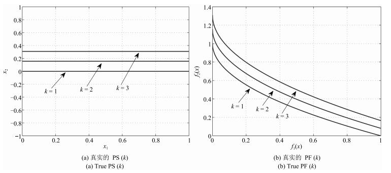
图 2 函数FDA3在三个时刻的真实Pareto解与前沿的比较
Fig. 2 True Pareto solutions and Pareto fronts of FDA3 in three environments
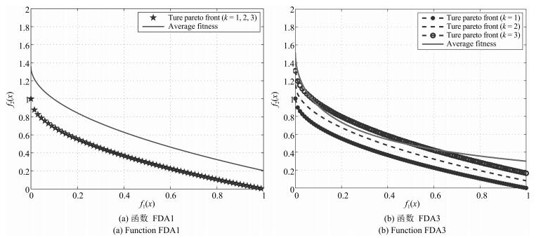
图 3 函数的平均适应度值与时刻$k=1, 2, 3$的真实Pareto前沿的比较
Fig. 3 Average fitness and true PF($k$) with $k=1, 2, 3$
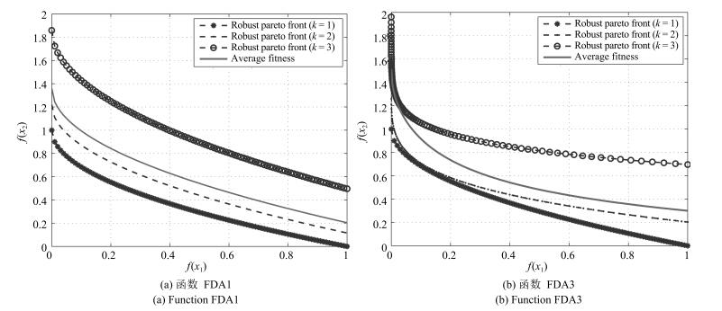
图 4 函数的平均适应度值与鲁棒解RPS在$t=1, 2, 3$时刻的鲁棒Pareto前沿的比较
Fig. 4 Average fitness and robust Pareto fronts with $k=1, 2, 3$
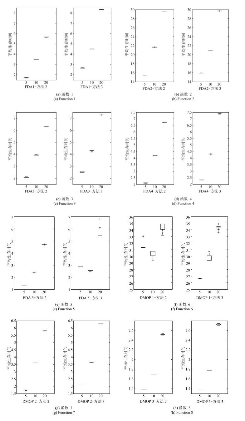
图 5 不同变化强度$n_{ d} =5, 10, 20$下方法2和方法3的平均生存时间比较($\eta=0.4$, $T=2$, $\tau _{ d} =30$)
Fig. 5 Average survival time of methods 2 and 3 in different change severity $n_{ d} =5, 10, 20$ ($\eta=0.4$, $T=2$, $\tau _{ d} =30$)
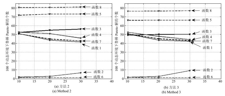
图 6 不同变化频率$\tau _{ d}=10, 20, 30$下方法2和方法3的平均生存时间比较($\eta =0.4$, $T=2$, $n_{ d} =10$)
Fig. 6 Average survival time of methods 2 and 3 in different change frequency $\tau _{ d}=10, 20, 30$ ($\eta =0.4$, $T=2$, $n_{ d} =10$)
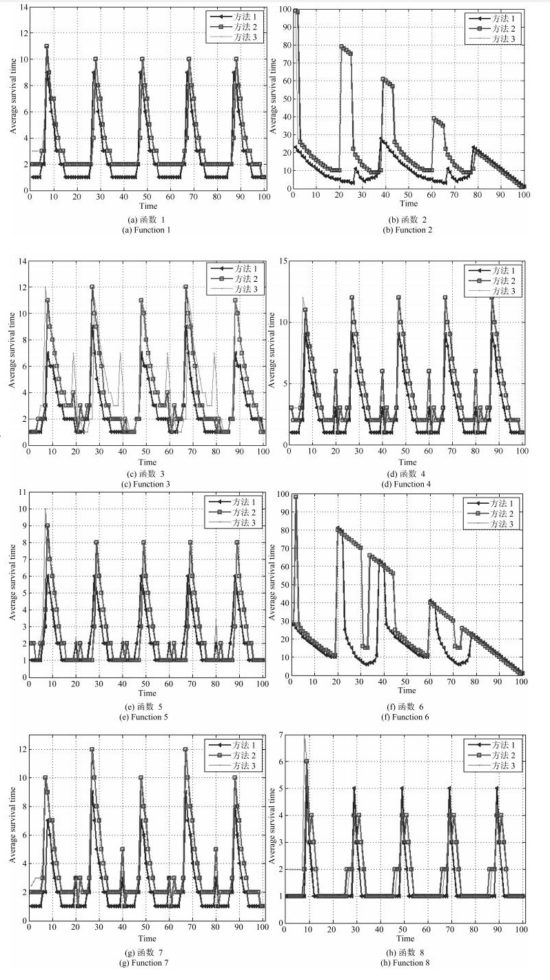
图 7 100个动态环境下三种方法的鲁棒生存时间比较$\eta=0.4$, $T=2$, $n_{ d} =10$, $\tau _{ d} =30$
Fig. 7 Robust survival time of three methods in 100 environments ($\eta =0.4$, $T=2$, $n_{ d} =10$, $\tau _{ d} =30$)
图 8 3种方法获得鲁棒Pareto解集的生存时间百分比比较($\eta =0.4$, $T=2$, $n_{ d}=10$, $\tau _{ d} =30$)
Fig. 8 Robust survival time percentage of three methods ($\eta =0.4$, $T=2$, $n_{ d}=10$, $\tau _{ d} =30$)
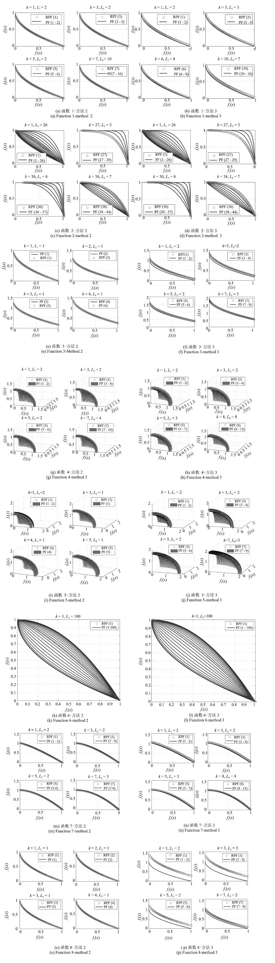
图 9 8个测试函数的前四个鲁棒Pareto解与其所适应的动态环境下的真实Pareto解的比较图\\ ($\eta=0.4$, $T=2$, $n_d =10$, $\tau _d =100$)
Fig. 9 The first four robust Pareto fronts and true Pareto fronts in their adaptive environments ($\eta=0.4$, $T=2$, $n_d =10$, $\tau _d =100$)
表 1 RPS(1)与相邻$k=2, 3$环境下解的相对适应度差值
Table 1 The relative fitness errors of RPS(1) and adjacent two environments
相对适应度差 $\Delta (1)$ $\Delta (2)$ FDA1 0.301 1.2177 FDA3 0.6728 1.7687  下载: 导出CSV
表 2 测试函数
Table 2 Benchmark functions
函数 测试函数 变量维数 变量范围 说明 Fun 1 $ f_1 (X_{Ⅰ})=x_1, \ f_2 =g\times h$
$g(X_{Ⅱ})=1+\sum_{x_i \in X_{Ⅱ}} {(x_i -G(k))^2}$
$ h(f_1, g)=1-\sqrt {{{f_1 }/ g}}, \ G(k)=\sin (0.5\pi k)$$ N=10$
$| X_{Ⅰ} | =1$
$| X_{Ⅱ} | $=9$ X_{Ⅰ} =(x_1)\in [0, 1]$
$X_{Ⅱ} =(x_2, {\cdots}, x_N)\in [-1, 1]$FDA1 in [6]
PS随环境变化
PF不随环境变化Fun 2 $f_1 (X_{Ⅰ})=x_1, f_2 =g\times h$
$g(X_{Ⅱ})=1+\sum_{x_i \in X_{Ⅱ} } {x_i^2 }$
$h(f_1, g)=1-\left({{{f_1 }/g}} \right)^{H(k)^{-1}}$
$H(k)=0.75+0.7\sin (0.5\pi k)$$ N=10$
$| X_{Ⅰ} | =1$
$| X_{Ⅱ} | =9$$X_\rm{1} =(x_1)\in [0, 1],$
$X_\rm{2} \in [-1, 1]$FDA2 in [6]
PS不随环境变化
PF随环境变化Fun 3 $ f_1 (X_{Ⅰ})=\sum_{x_i \in X_\rm{1} }^n {x_i^{F(k)} }, \quad f_2 =g\times h$
$g(X_{Ⅱ})=1+G(k)+\sum_{x_i \in X_{Ⅱ}}{(x_i -G(k))^2}$
$h(f_1, g)=1-\sqrt {{{f_1 }/g}}, \quad G(k)=\left| {\sin (0.5\pi k)} \right|$
$F(k)=10^{2\sin (0.5\pi k)}$$ N=10$
$| X_{Ⅰ} | =1$
$| X_{Ⅱ} |$ =9$X_{Ⅰ}=(x_1)\in [0, 1]$
$X_{Ⅱ} =(x_2, {\cdots}, x_N)\in [-1, 1]$FDA3 in [6]
PS随环境变化
PF随环境变化Fun 4 $ f_1 (x)=(1+g)\cos (0.5\pi x_1)\cos (0.5\pi x_2)$
$f_2 (x)=(1+g)\cos (0.5\pi x_1)\sin (0.5\pi x_2)$
$f_3 (x)=(1+g)\sin (0.5\pi x_1)$
$g(x)=\sum_{i=3}^n {(x_i -G(k))^2}$
$G(k)=\left| {\sin (0.5\pi t)} \right|$$N=12$ $ x_i \in [0, 1]$
$\forall\, i=1, 2, {\cdots}, N $FDA4 in [6]
PS随环境变化
PF不随环境变化Fun 5 $ f_1 (x)=(1+g)\cos (0.5\pi y_1)\cos (0.5\pi y_2)$
$f_2 (x)=(1+g)\cos (0.5\pi y_1)\sin (0.5\pi y_2)$
$f_3 (x)=(1+g)\sin (0.5\pi y_1)$
$g(x)=G(k)+\sum_{i=3}^n {(x_i -G(k))^2}$
$y_i =x_i^{F(k)}$
$G(k)=\left| {\sin (0.5\pi k)} \right|$
$F(k)=1+100\sin ^4(0.5\pi k)$$N=12$ $ x_i \in [0, 1]$
$\forall\, i=1, 2, {\cdots}, N $FDA5 in [6]
PS随环境变化
PF随环境变化Fun 6 $ f_1 (x_1)=x_1, f_2 =g\times h$
$g(x_2, {\cdots}, x_n, k)=1+9\sum_{i=2}^n {x_i^2 }$
$h(f_1, g)=1-\left({{{f_1 } /g}} \right)^{H(k)}$
$H(k)=0.75\sin (0.5\pi k)$+1.25$N=10$ $ x_i \in [0, 1]$
$\forall\, i=1, 2, {\cdots}, N $DMOP1 in [8]
PS不随环境变化
PF随环境变化Fun 7 $ f_1 (x_1)=x_1, f_2 =g\times h$
$g(x_2, {\cdots}, x_n, k)=1+\sum_{i=2}^n {(x_i -G(k))^2}$
$h(f_1, g)=1-\left({{{f_1 }/g}} \right)^{H(k)}$
$H(k)=0.75\sin (0.5\pi k)$+1.25$N=10$ $ x_i \in [0, 1]$
$\forall\, i=1, 2, {\cdots}, N $DMOP2 in [8]
PS随环境变化
PF随环境变化Fun 8 $f_1 (x_1)=x_1, f_2 =g\times h$
$g(x_2, {\cdots}, x_n, k)=1+9\sum_{i=2}^n {(x_i -G(k))^2}$
$h(f_1, g)=1-\sqrt {{{f_1 } / g}}$
$H(t)=\sin (0.5\pi k)$$N=10$ $ x_i \in [0, 1]$
$\forall\, i=1, 2, {\cdots}, N $DMOP3 in [8]
PS随环境变化
PF不随环境变化
下载: 导出CSV
表 3 不同稳定性阈值下两种模型的平均生存时间比较($T=2$, $n_{ d} =10$, $\tau_{ d} =30$)
Table 3 Average survival time of methods 2 and 3 in different stability thresholds ($T=2$, $n_{ d} =10$, $\tau_{ d} =30$)
方法 参数 函数1 函数2 函数3 函数4 函数5 函数6 函数7 函数8 方法2 $\eta =0.2$ 2.4480±0.0314 7.2233±0.0082 2.3433±0.0342 2.6867±0.0049 1.6120±0.0041 9.9680±0.0041 2.2813±0.0106 1.2407±0.0110 $\eta=0.4$ 3.4640±0.0099 21.658±0.0086 3.9428±0.0208 4.2027±0.0096 2.4093±0.0026 30.197±0.5440 3.6000±9.1E-16 1.7000±7.3E-15 $\eta=0.6$ ${\bf 4.5720\pm0.0077}$ ${\bf 49.51\pm0} $ $ {\bf 5.9933\pm0.0049} $ ${\bf 6.1293\pm0.0080}$ $ {\bf 4.3727\pm0.0059} $ $ {\bf 49.510\pm0} $ $ {\bf 4.8247\pm0.0210} $ $ {\bf 2.2867\pm0.0105}$ 方法3 $\eta=0.2$ 2.5067±0.0315 7.4120±0.2402 2.5500±0.0746 2.7800±9.1E-16 1.7200±2.2E-16 9.9453±0.0074 2.3347±0.0106 1.2600±2.2E-16 $\eta=0.4$ 3.5133±0.0082 20.941±0.0083 4.3147±0.0280 4.3187±0.0106 2.5500±0.0318 30.007±0.4951 3.6520±0.0068 1.7800±4.6E-16 $\eta=0.6$ ${\bf 4.5940\pm0.0019}$ $ {\bf 49.510\pm0} $ $ {\bf 6.1227\pm0.0046} $ $ {\bf 6.2727\pm0.0110} $ $ {\bf 4.4787\pm0.0035} $ $ {\bf 49.510\pm0} $ $ {\bf 4.8607\pm0.0026} $ $ {\bf 2.4033\pm0.0082}$
下载: 导出CSV
表 4 不同时间窗下两种模型的平均生存时间比较($\eta =0.4$, $n_{ d} =10$, $\tau_{ d} =30$)
Table 4 Average survival time of methods 2 and 3 in different time windows ($\eta =0.4$, $n_{ d} =10$, $\tau_{ d} =30$)
方法 参数 函数1 函数2 函数3 函数4 函数5 函数6 函数7 函数8 方法2 $T=2 $ $ {\bf 3.4640\pm0.0099} $ $ {\bf 21.658\pm0.0086} $ 3.9428±0.0208 $ {\bf 4.2027\pm0.0096}$ 2.4093±0.0026 $ {\bf 30.197\pm0.5440} $ $ {\bf 3.6000\pm9.1}$E-${\bf 16}$ $ {\bf 1.7000\pm7.3}$E-${\bf 15}$ $T=4 $ 3.1460±0.0051 21.606±0.1788 3.6447±0.0168 3.9440±0.0203 $ {\bf 2.4500\pm0.0038} $ 29.448±0.7324 3.1707±0.0406 1.5220±0.0056 $T=6 $ $ 3.1180\pm0.0115 $ $ 21.650\pm3.6$E-15 $ {\bf 4.0373\pm0.0059} $ $ 3.9007\pm0.0167$ $ {{\bf 2.4500\pm0}} $ 29.085±0.6836 3.2027±0.0448 1.5220±0.0056 方法3 $T=2 $ $ {\bf 3.5133\pm0.0082} $ $ {\bf 20.941\pm0.0083} $ $ {\bf 4.3147\pm0.0280} $ $ {\bf 4.3187\pm0.0106}$ 2.5500±0.0318 $ {\bf 30.007\pm0.4951} $ $ {\bf 3.6520\pm0.0068} $ $ {\bf 1.7800\pm4.6}$E$-{\bf 16}$ $T=4 $ 3.4033±0.0082 20.900±0 3.9533±0.0082 4.1893±0.0110 2.7100±4.5E-16 28.068±0.2995 3.3927±0.0546 1.5600±2.2E-16 $T=6 $ 3.4120±0.0108 20.644±0.3445 4.1467±0.0374 4.2313±0.0125 $ {\bf 2.8813\pm0.0376} $ 28.340±0.4003 3.4820±0.0441 1.5940±0.0356
下载: 导出CSV
表 5 不同时间窗下两种模型的RIGD测度比较($\eta =0.4$, $n_{ d} =10$, $\tau_{ d} =30$)
Table 5 RIGD of methods 2 and 3 in different time windows ($\eta =0.4$, $n_{ d} =10$, $\tau_{ d} =30$)
方法 参数 函数1 函数2 函数3 函数4 函数5 函数6 函数7 函数8 方法2 $T=2$ $ 0.2267\pm0.0092 $ $ {\bf 0.0816\pm0.0555} $ $ {\bf 0.3815\pm0.0230} $ $ 0.4009\pm0.0178$ $ {\bf 0.4638\pm0.0218} $ $ 0.1009\pm0.0754 $ $ 0.3476\pm0.0132 $ $ 2.5449\pm0.1079$ $T=4$ $ {\bf 0.1944\pm0.0081} $ $ 0.1364\pm0.0911 $ $ 0.4142\pm0.0296 $ $ 0.4009\pm0.0177$ $ 0.5424\pm0.0250 $ $ {\bf 0.0707\pm0.0323} $ $ {\bf 0.3306\pm0.0171} $ $ 2.1396\pm0.0972$ $T=6$ $ 0.2270\pm0.0077 $ $ 0.1552\pm0.1226 $ $ 0.8548\pm0.1841 $ $ {\bf 0.4008\pm0.0200} $ $ 0.7334\pm0.0571 $ $ 0.0928\pm0.0457 $ $ 0.3476\pm0.0181 $ $ {\bf 2.0528\pm0.0880}$ 方法3 $T=2$ $ 0.2276\pm0.0063 $ $ {\bf 0.0849\pm0.0559} $ $ {\bf 0.3842\pm0.0215} $ $ 0.4520\pm0.0169$ $ {\bf 0.5907\pm0.0444} $ $ {\bf 0.0811\pm0.0543} $ $ 0.3477\pm0.0128 $ $ {\bf 2.5629\pm0.0999}$ $T=4$ $ {\bf 0.1976\pm0.0066} $ $ 0.2238\pm0.1382 $ $ 0.5184\pm0.1738 $ $ {\bf 0.4057\pm0.0070}$ $ 0.7655\pm0.0278 $ $ 0.1168\pm0.1083 $ $ {\bf 0.3328\pm0.0089} $ $ 3.4348\pm0.1043$ $T=6$ $ 0.5411\pm0.1200 $ $ 0.1432\pm0.0457 $ $ 1.2358\pm0.0851 $ $ 0.6615\pm0.0048 $ $ 1.2572\pm0.1641 $ $ 0.1812\pm0.0857 $ $ 0.9319\pm0.0289 $ $ 11.416\pm0.2446 $
下载: 导出CSV
表 6 三种方法获得鲁棒Pareto解集的平均生存时间比较($\eta =0.4$, $T=2$, $n_{ d}=10$, $\tau _{ d} =30$)
Table 6 Average survival time of robust Pareto solutions on three methods ($\eta =0.4$, $T=2$, $n_{ d}=10$, $\tau _{ d} =30$)
方法 函数1 函数2 函数3 函数4 函数5 函数6 函数7 函数8 方法1 2.5800±0.0086 10.090±0.1376 2.6200±0.3880 2.7300±0.6077 2.9900±0.0560 17.940±0.8734 2.2400±0.3525 1.3500±3.6E-15 方法2 3.4640±0.0099 $ {\bf 21.658\pm0.0086} $ 3.9428±0.0208 4.2027±0.0096 $2.4093\pm0.0026 $ $ {\bf 30.197\pm0.5440} $ 3.6000±9.1E-16 1.7000±7.3E-15 方法3 ${\bf 4.5073\pm0.0133} $ 20.941±0.0083 $ {\bf 4.3147\pm0.0280} $ $ {\bf 4.3187\pm0.0106}$ ${\bf 2.5500\pm0.0318} $ 30.007±0.4951 $ {\bf 3.6520\pm0.0068} $ $ {\bf 1.7800\pm4.6}$E-${\bf 16}$
下载: 导出CSV
表 7 三种方法获得鲁棒Pareto解集的RIGD测度比较($\eta =0.4$, $T=2$, $n_{ d}=10$, $\tau _{ d} =30$)
Table 7 RIGD of robust Pareto solutions on three methods ($\eta =0.4$, $T=2$, $n_{ d}=10$, $\tau _{ d} =30$)
方法 函数1 函数2 函数3 函数4 函数5 函数6 函数7 函数8 方法1 ${\bf 0.0095\pm0.0021} $ 0.2438±0.0316 $ {\bf 0.1544\pm0.0579} $ $ {\bf 0.0543\pm0.0043}$ ${\bf 0.3619\pm0.1683} $ 0.1564±1.04E-7 $ {\bf 0.1335\pm0.0743} $ $ {\bf 0.1866\pm1.40}$E-${\bf 6}$ 方法2 0.2267±0.0092 $ {\bf 0.0816\pm0.0555} $ 0.3815±0.0230 0.4009±0.0178 0.4638±0.0218 0.1009±0.0754 0.3476±0.0132 2.5449±0.1079 方法3 0.2276±0.0063 0.0849±0.0559 0.3842±0.0215 0.4520±0.0169 0.5907±0.0444 $ {\bf 0.0811\pm0.0543} $ 0.3477±0.0128 2.5629±0.0999
下载: 导出CSV
表 8 三种方法求解鲁棒Pareto最优解的平均运行时间(s)比较($\eta=0.4$, $T=2$, $n_{ d} =10$, $\tau _{ d} =30$)
Table 8 Average elapsed time of robust Pareto solutions on three methods ($\eta=0.4$, $T=2$, $n_{ d} =10$, $\tau _{ d} =30$)
方法 函数1 函数2 函数3 函数4 函数5 函数6 函数7 函数8 方法1 51.3681±3.4762 13.2158±4.0439 70.8508±1.2940 185.9928±10.9027 710.6224±70.2617 1.7005±0.0077 54.8422±2.6081 128.4283±2.3889 方法2 ${\bf 46.0068\pm1.4818} $ $ {\bf 7.0358\pm4.2498} $ 59.0582±1.1731 $ {\bf 172.3075\pm7.6934}$ ${\bf 315.2275\pm8.4846} $ $ {\bf 0.8673\pm0.0140} $ $ {\bf 45.7206\pm2.3813} $ 89.7115±0.9206 方法3 49.3816±1.8679 10.2509±3.2404 $ {\bf 55.8101\pm2.2671} $ 190.0556±19.8364 340.7134±21.4715 1.0038±0.0046 47.8325±2.0709 $ {\bf 84.1739\pm0.8742}$
下载: 导出CSV
-
[1] Farina M, Deb K, Amato P. Dynamic multiobjective optimization problems:test cases, approximations, and applications. IEEE Transactions on Evolutionary Computation, 2004, 8(5):425-442 doi: 10.1109/TEVC.2004.831456 [2] 刘敏, 曾文华.记忆增强的动态多目标分解进化算法.软件学报, 2013, 24(7):1571-1588 http://d.wanfangdata.com.cn/Periodical/rjxb201307011Liu Min, Zeng Wen-Hua. Memory enhanced dynamic multi-objective evolutionary algorithm based on decomposition. Journal of Software, 2013, 24(7):1571-1588 http://d.wanfangdata.com.cn/Periodical/rjxb201307011 [3] Hatzakis I, Wallace D. Dynamic multi-objective optimization with evolutionary algorithms:a forward-looking approach. In:Proceedings of the 8th Annual Conference on Genetic and Evolutionary Computation. New York, USA:ACM, 2006. 1201-1208 http://dl.acm.org/citation.cfm?id=1144187 [4] Zhou A M, Jin Y C, Zhang Q F, Sendhoff B, Tsang E. Prediction-based population re-initialization for evolutionary dynamic multi-objective optimization. In:Proceedings of the 4th International Conference on Evolutionary Multi-Criterion Optimization. Berlin Heidelberg, Germany:Springer, 2007. 832-846 http://dl.acm.org/citation.cfm?id=1762615 [5] Zhou A M, Jin Y C, Zhang Q F. A population prediction strategy for evolutionary dynamic multiobjective optimization. IEEE Transactions on Cybernetics, 2014, 44(1):40-53 doi: 10.1109/TCYB.2013.2245892 [6] Goh C K, Tan K C. A competitive-cooperative coevolutionary paradigm for dynamic multiobjective optimization. IEEE Transactions on Evolutionary Computation, 2009, 13(1):103-127 doi: 10.1109/TEVC.2008.920671 [7] 胡成玉, 姚宏, 颜雪松.基于多粒子群协同的动态多目标优化算法及应用.计算机研究与发展, 2013, 50(6):1313-1323 doi: 10.7544/issn1000-1239.2013.20110847Hu Cheng-Yu, Yao Hong, Yan Xue-Song. Multiple particle swarms coevolutionary algorithm for dynamic multi-objective optimization problems and its application. Journal of Computer Research and Development, 2013, 50(6):1313-1323 doi: 10.7544/issn1000-1239.2013.20110847 [8] Jin Y C, Sendhof B. Constructing dynamic optimization test problems using the multi-objective optimization concept. Applications of Evolutionary Computing. Berlin Heidelberg, Germany:Springer, 2004. 525-536 doi: 10.1007/978-3-540-24653-4_53 [9] Nguyen T T, Yang S S, Branke J. Evolutionary dynamic optimization:a survey of the state of the art. Swarm and Evolutionary Computation, 20126:1-24 doi: 10.1016/j.swevo.2012.05.001 [10] Camara M, Ortega J, de Toro F. A single front genetic algorithm for parallel multi-objective optimization in dynamic environments. Neurocomputing, 2009, 72(16-18):3570-3579 doi: 10.1016/j.neucom.2008.12.041 [11] Deb K, Gupta H. Introducing robustness in multi-objective optimization. Evolutionary Computation, 2006, 14(4):463-494 doi: 10.1162/evco.2006.14.4.463 [12] Yu X, Jin Y C, Tang K, Yao X. Robust optimization over time——a new perspective on dynamic optimization problems. In:Proceedings of the 2010 IEEE Congress on Evolutionary Computation. Barcelona, Spain:IEEE, 2010. 1-6 doi: 10.1109/cec.2010.5586024 [13] Jin Y C, Tang K, Yu X, Sendhoff B, Yao X. A framework for finding robust optimal solutions over time. Memetic Computing, 2013, 5(1):3-18 doi: 10.1007/s12293-012-0090-2 [14] Fu H B, Sendhoff B, Tang K, Yao X. Finding robust solutions to dynamic optimization problems. Lecture Notes in Computer Science, 2013, 7835:616-625 doi: 10.1007/978-3-642-37192-9 [15] Fu H B, Sendhoff B, Tang K, Yao X. Robust optimization over time:problem difficulties and benchmark problems. IEEE Transactions on Evolutionary Computation, 2015, 19(5):731-745 doi: 10.1109/TEVC.2014.2377125 [16] Chen M R, Guo Y N, Liu H Y. The evolutionary algorithm to find robust Pareto-optimal solutions over time. Mathematical Problems in Engineering, 2015, 2015:Article ID 814210 doi: 10.1155/2015/814210 [17] Zhang Q F, Li H. MOEA/D:a multiobjective evolutionary algorithm based on decomposition. IEEE Transactions on Evolutionary Computation, 2007, 11(6):712-731 doi: 10.1109/TEVC.2007.892759 [18] Jan M A, Khanum R A. A study of two penalty-parameterless constraint handling techniques in the framework of MOEA/D. Applied Soft Computing, 2013, 13(1):128-148 doi: 10.1016/j.asoc.2012.07.027 [19] 何书元.应用时间序列分析.北京:北京大学出版社, 2003.He Shu-Yuan. Time Series Analysis. Beijing:Peking University Press, 2003. -

 下载:
下载:

计量
- 文章访问数: 3578
- HTML全文浏览量: 482
- PDF下载量: 699
- 被引次数: 0
