

A Many-objective Evolutionary Algorithm Based on Weighted Sum of Objective Space Transformation
-
摘要: 权重求和是基于分解的超多目标进化算法中常用的方法, 相比其他方法具有计算简单、搜索效率高等优点, 但难以有效处理帕累托前沿面(Pareto optimal front, PF)为非凸型的问题. 为充分发挥权重求和方法的优势, 同时又能处理好PF为非凸型的问题, 本文提出了一种基于目标空间转换权重求和的超多目标进化算法, 简称NSGAIII-OSTWS. 该算法的核心是将各种问题的PF转换为凸型曲面, 再利用权重求和方法进行优化. 具体地, 首先利用预估PF的形状计算个体到预估PF的距离; 然后, 根据该距离值将个体映射到目标空间中预估凸型曲面与理想点之间的对应位置; 最后, 采用权重求和函数计算出映射后个体的适应值, 据此实现对问题的进化优化. 为验证NSGAIII-OSTWS的有效性, 将NSGAIII-OSTWS与7个NSGAIII的变体, 以及9个具有代表性的先进超多目标进化算法在WFG、DTLZ和LSMOP基准问题上进行对比, 实验结果表明NSGAIII-OSTWS具备明显的竞争性能.Abstract: The weighted sum method is a common decomposition method in many-objective evolutionary algorithm based on decomposition. Compared with other methods, it has the advantages of computationally easy and high search efficiency. However, it is difficult for this method to handle the problem with nonconvex Pareto optimal front (PF) effectively. To take full advantage of the weighted sum method and effectively handle the problem with nonconvex PF at the same time, a many-objective evolutionary algorithm based on weighted sum of objective space transformation is proposed, namely NSGAIII-OSTWS. The core of the NSGAIII-OSTWS is to transform the PF of various problems into convex surfaces, and then apply the weighted sum method to optimize the transformed problem. Specifically, the distance between the individual and the estimated PF is calculated firstly. Then all individuals are mapped into the corresponding location between the estimated convex surface and the ideal point according to their distance value. Finally, the fitness values of all mapped individuals are calculated by weighted sum function, and then the evolutionary optimization of the problem is proceeded. In order to verify the effectiveness of NSGAIII-OSTWS, seven variants of NSGAIII, and nine representative advanced many-objective evolutionary algorithms are compared on the WFG, DTLZ and LSMOP benchmark problems. The experimental results show that NSGAIII-OSTWS has obviously competitive performance compared with the comparison algorithms.1) 收稿日期 2020-06-30 录用日期 2021-01-26 Manuscript received June 30, 2020; accepted January 26, 2021 国家重点研发计划(2021YFB2900800), 国家自然科学基金(61871272), 广东省自然科学基金(2021A1515011911, 2020A1515010479), 深圳市科技计划(20200811181752003, GGFW2018020518310863)资助 Supported by National Key Research and Development Program of China (2021YFB2900800), National Natural Science Foundation of China (61871272), Natural Science Foundation of Guangdong, China (2021A1515011911, 2020A1515010479), Shenzhen Scientific Research and Development Funding Program (20200811181752003, GGFW2018020518310863) 本文责任编委 李成栋 Recommended by Associate Editor LI Cheng-Dong2) 1. 深圳大学计算机与软件学院 深圳 518060 2. 深圳大学信息 中心 深圳 518060 1. College of Computer Science and Software Engineering, Shenzhen University, Shenzhen 518060 2. Information Center, Shenzhen University, Shenzhen 518060
-
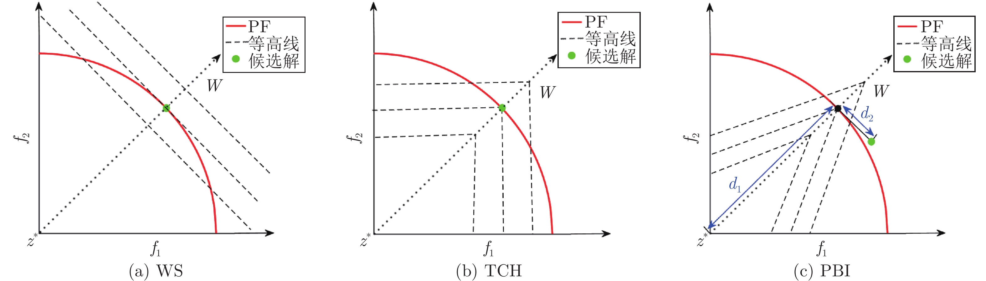
图 1 分解方法WS, TCH和PBI在参考向量w上的二维示意图, 其中虚线为等高线
Fig. 1 Illustration of the decomposition methods WS, TCH and PBI on reference vector w, where dashed lines are contour lines
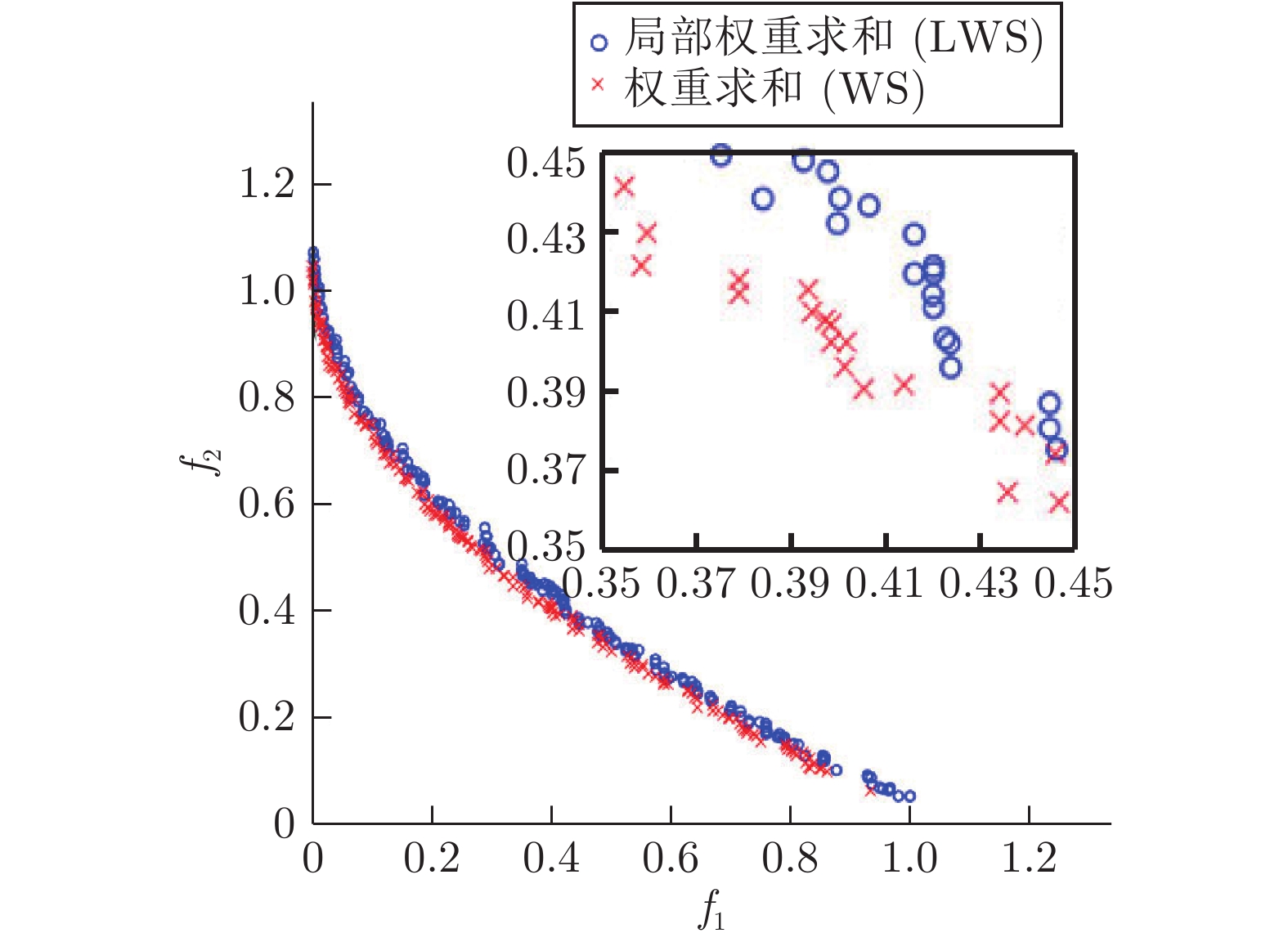
图 2 NSGAIII-WS和NSGAIII-LWS算法在ZDT1上获得的最终种群分布
Fig. 2 The final population distribution obtained by NSGAIII-WS and NSGAIII-LWS algorithm on ZDT1
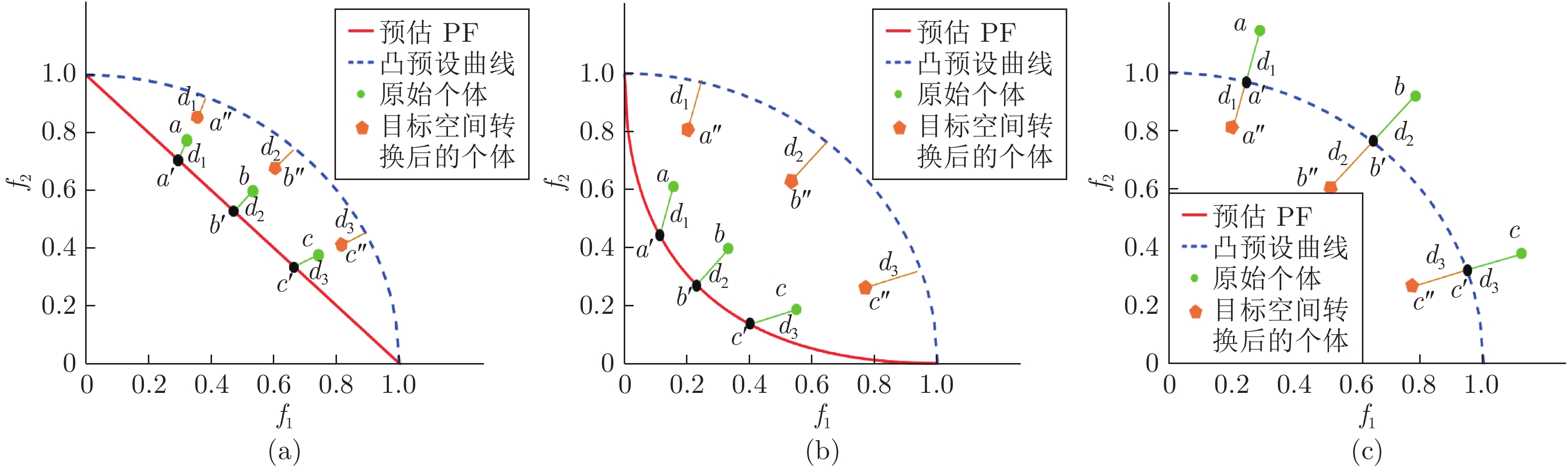
图 3 OSTWS方法将PF形状为线形(a), 凸形(b)和凹形(c)种群中的个体转换到凸目标空间的整个过程
Fig. 3 The whole process of transforming the population individuals from linear (a), convex (b) and concave (c) into convex objective space by OSTWS method
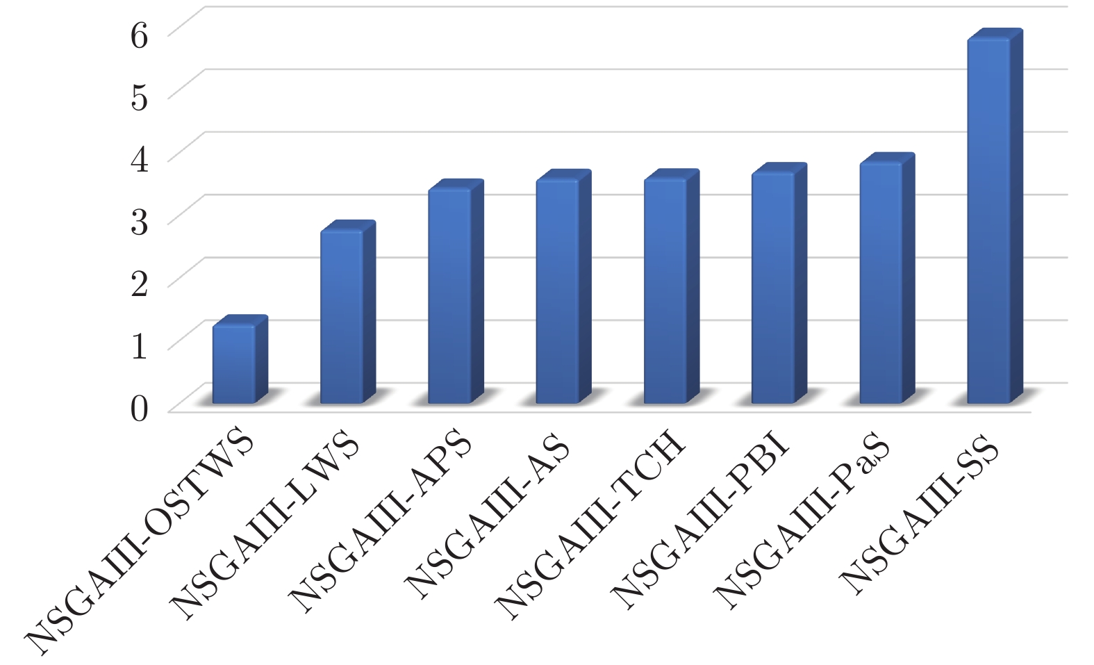
图 4 NSGAIII-OSTWS, NSGAIII-LWS, NSGAIII-TCH, NSGAIII-PBI, NSGAIII-AS, NSGAIII-SS, NSGAIII-APS和NSGAIII-PaS, 在所有测试问题实例中的平均IGD+性能得分排名. 得分越小, 整体性能越好
Fig. 4 Ranking in the average performance score over all test problem instances for the algorithms of NSGAIII-OSTWS, NSGAIII-LWS, NSGAIII-TCH, NSGAIII-PBI, NSGAIII-AS, NSGAIII-SS, NSGAIII-APS and NSGAIII-PaS. The smaller the score, the better the overall performance in terms of IGD+
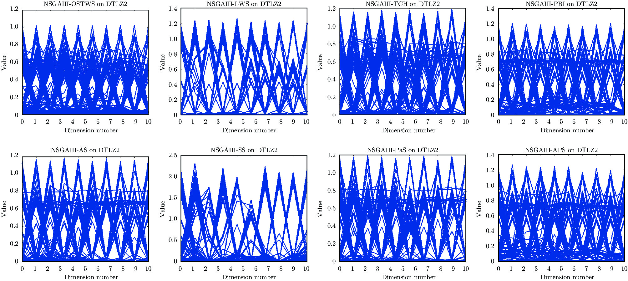
图 5 NSGAIII-OSTWS, NSGAIII-LWS, NSGAIII-TCH, NSGAIII-PBI, NSGAIII-AS, NSGAIII-SS, NSGAIII-PaS和NSGAIII-APS在10维DTLZ2问题上所获得的解集
Fig. 5 Solution set of NSGAIII-OSTWS, NSGAIII-LWS, NSGAIII-TCH, NSGAIII-PBI, NSGAIII-AS, NSGAIII-SS, NSGAIII-PaS and NSGAIII-APS on DTLZ2 problem with 10-objectives
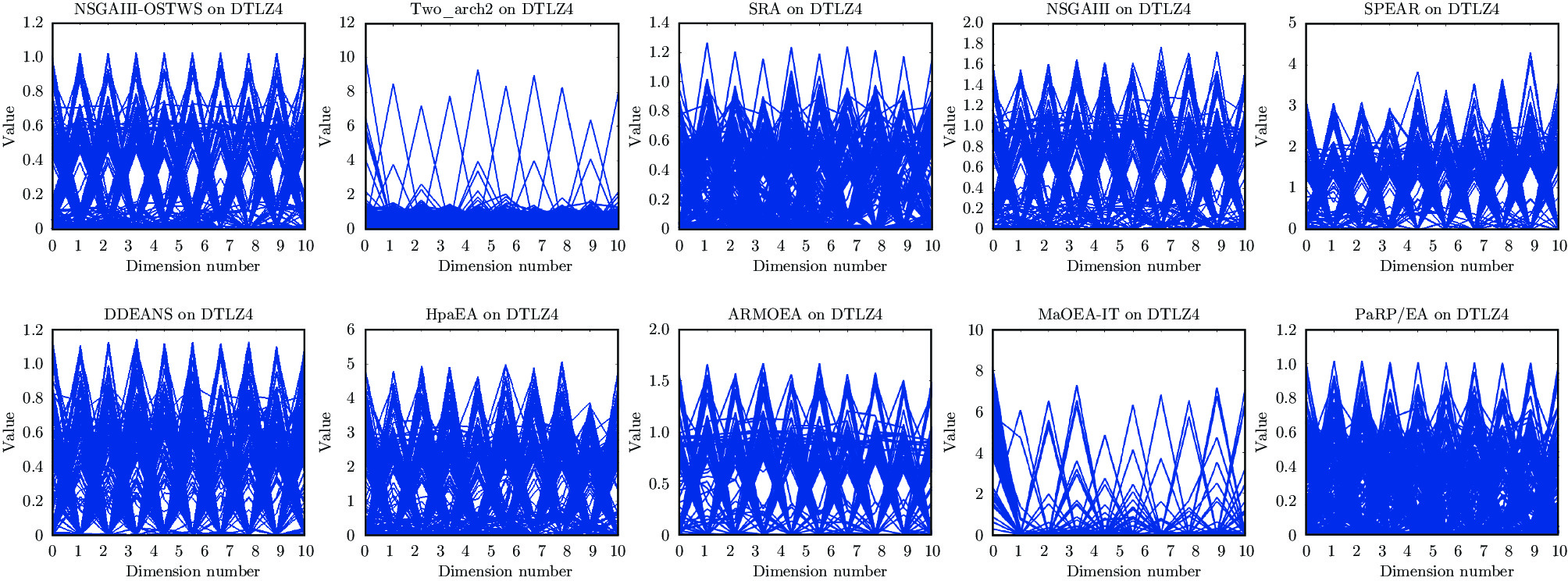
图 6 SRA, SPEAR, DDEANS, HpaEA, ARMOEA, MaOEA-IT和PaRP/EA在10维DTLZ4问题上所获得的解集
Fig. 6 Solution set of NSGAIII-OSTWS, NSGAIII, Two_arch2, SRA, SPEAR, DDEANS HpaEA, ARMOEA, MaOEA-IT and PaRP/EA on DTLZ4 problem with 10-objectives
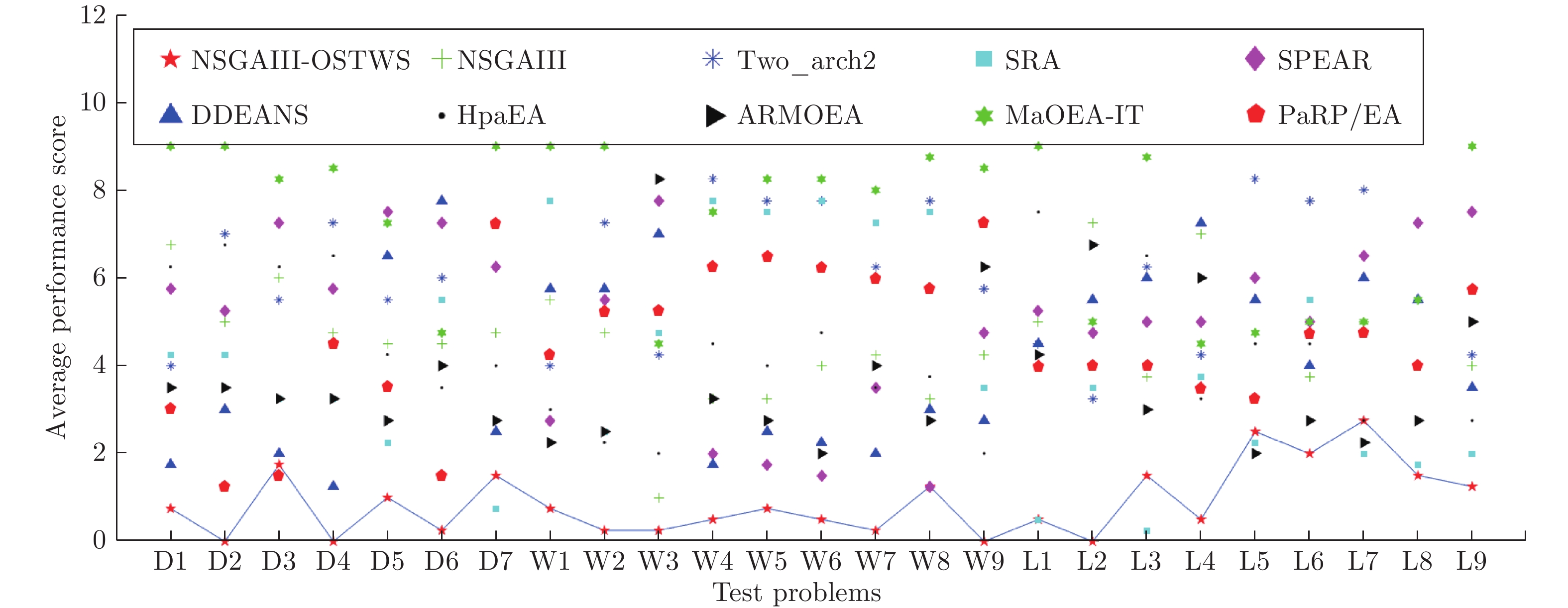
图 7 NSGAIII-OSTWS, NSGAIII, Two_arch2, SRA, SPEAR, DDEANS, HpaEA, ARMOEA, MaOEA-IT和PaRP/EA在所有测试问题, 即DTLZ(Dx), WFG(Wx) 和LSMOP(Lx) 上的平均GD表现分, 分值越小, 算法的整体性能越好. 通过实线连接NSGAIII-OSTWS的得分, 以便易于评估分数
Fig. 7 Average performance score of NSGAIII-OSTWS, NSGAIII, Two_arch2, SRA, SPEAR, DDEANS, HpaEA, ARMOEA, MaOEA-IT and PaRP/EA on all test problems, namely DTLZ(Dx), WFG(Wx)and LSMOP(Lx). The smaller the score, the better the overall performance in terms of GD. The values of NSGAIII-OSTWS are connected by a solid line to easier assess the score
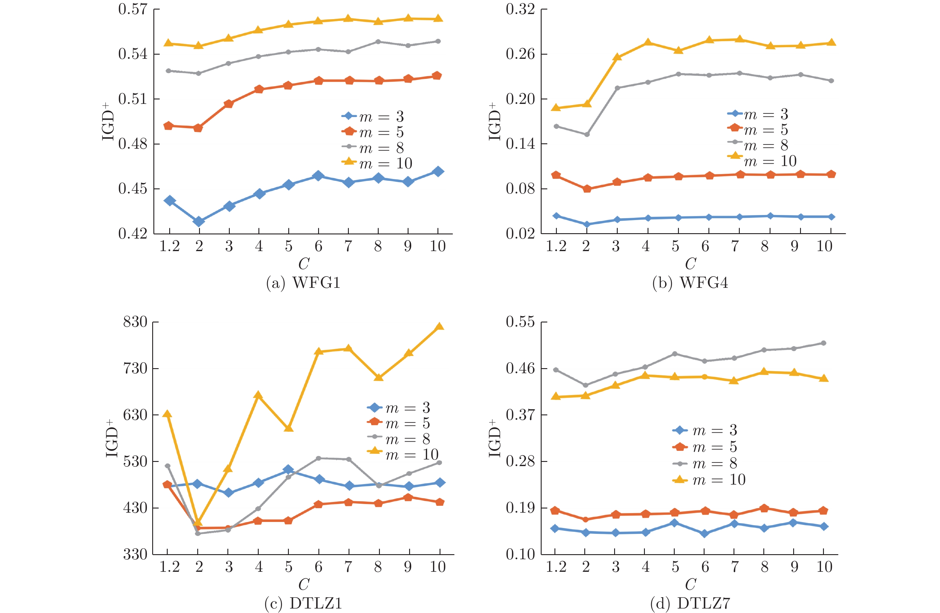
图 9 不同
$ C $ 值在WFG1, WFG4, DTLZ1和DTLZ7问题的3, 5, 8和10目标维度上的IGD+均值Fig. 9 The median IGD+ values of different
$ C $ values on WFG1, WFG4, DTLZ1 and DTLZ7 problems with 3-, 5-, 8-, and 10-objectives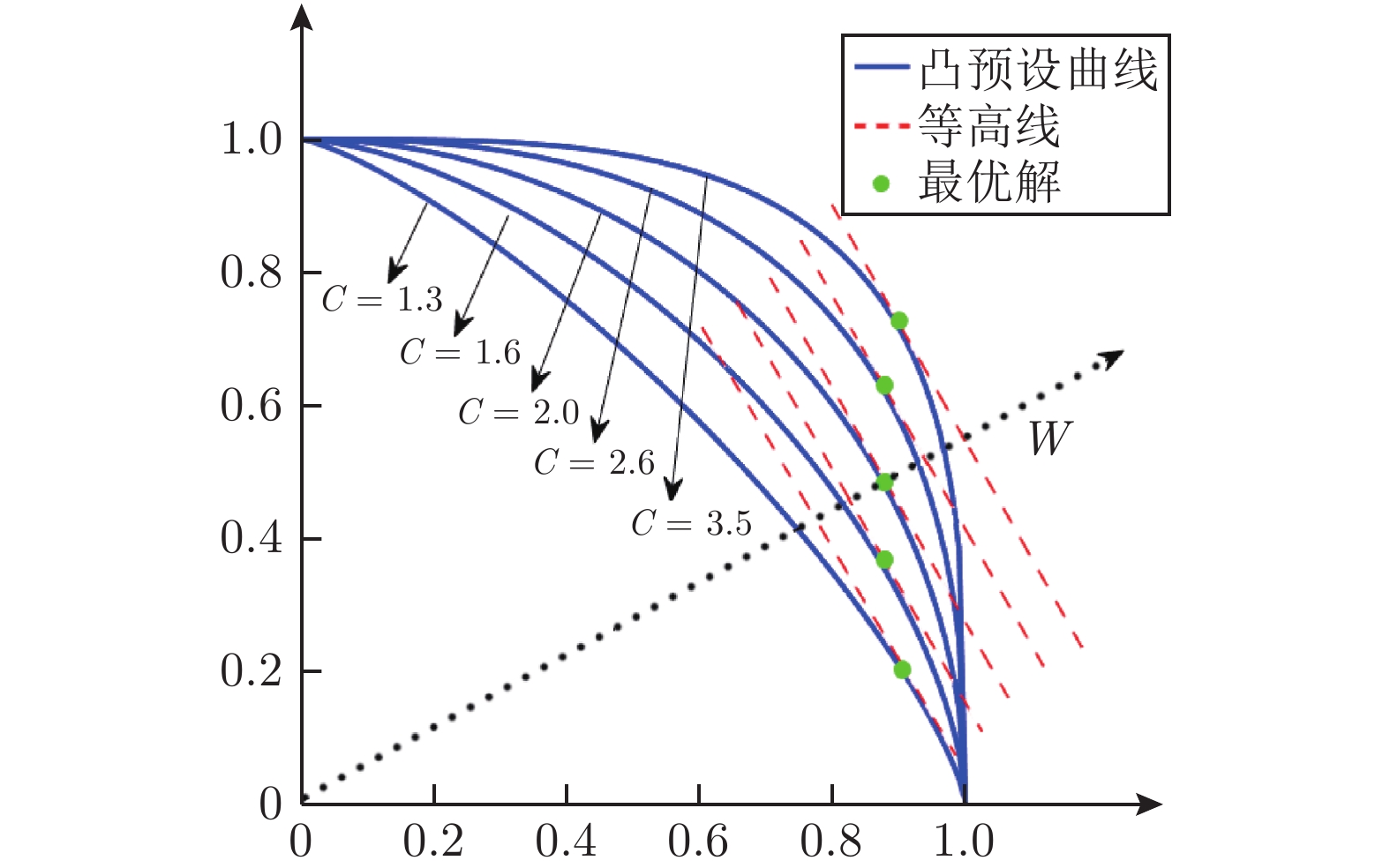
图 8 不同预设凸曲线在参考向量w上获得的最优解示意图
Fig. 8 The optimal solution obtained by different preset convex curves on the reference vector w
表 1 种群大小设置
Table 1 Setting of the population size
目标数 ($ m $) 分割数 ($ H $) 种群大小 ($ N $) 3 12 91 5 6 210 8 3, 2 156 10 3, 2 275  下载: 导出CSV
表 2 交叉变异参数设置
Table 2 Parameter settings for crossover and mutation
参数名 参数值 交叉概率 ($ P_c $) 1.0 变异概率 ($ P_m $) 1/$ D $ 交叉分布指标 ($ \eta_c $) 20 变异分布指标 ($ \eta_m $) 20
下载: 导出CSV
表 3 OSTWS, LWS, TCH, PBI, AS, SS, PaS和APS方法在框架为NSGAIII, 测试问题为DTLZ1-7上获得的GD值统计结果(均值和标准差). 每个实例算法中的最好结果以加粗突出显示
Table 3 The statistical results (mean and standard deviation) of the GD values obtained by OSTWS, LWS, TCH, PBI, AS, SS, PaS and APS methods on the NSGAIII framework and DTLZ1-7 test problems. The best average value among the algorithms for each instance is highlighted in bold
Problem $m$ NSGAIII-OSTWS NSGAIII-LWS NSGAIII-TCH NSGAIII-PBI NSGAIII-AS NSGAIII- SS NSGAIII-PaS NSGAIII-APS DTLZ1 3 6.915×101 7.734×101 7.411×101 7.140×101 7.678×101 7.749×101 7.554×101 7.376×101 (1.2×101) (9.4×100)− (9.3×100)$\approx$ (1.1×101)$\approx$ (1.1×101)− (7.3×100)− (9.4×100)$\approx$ (9.8×100)$\approx$ 5 4.218×101 7.562×101 8.102×101 7.015×101 7.870×101 1.294×10² 7.993×101 6.507×101 (4.5×100) (6.6×100)− (8.9×100)− (7.6×100)− (8.1×100)− (9.7×100)− (8.0×100)− (7.6×100)− 8 4.881×101 9.120×101 7.814×101 9.002×101 7.875×101 2.458×10² 7.411×101 8.732×101 (1.2×101) (7.3×100)− (1.1×101)− (1.1×101)− (1.2×101)− (5.8×101)− (9.0×100)− (8.8×100)− 10 4.422×101 9.338×101 7.014×101 7.334×101 6.757×101 2.672×10² 7.299×101 7.538×101 (1.8×101) (4.9×100)− (8.2×100)− (2.4×101)− (5.3×100)− (5.1×101)− (7.3×100)− (3.2×101)− DTLZ2 3 1.681×10⁻³ 3.971×10⁻³ 3.465×10⁻³ 4.582×10⁻³ 3.552×10⁻³ 6.753×10⁻³ 3.585×10⁻³ 4.529×10⁻³ (2.3×10⁻⁴) (6.1×10⁻⁴)− (3.9×10⁻⁴)− (6.8×10⁻⁴)− (4.2×10⁻⁴)− (1.1×10⁻³)− (5.2×10⁻⁴)− (6.4×10⁻⁴)− 5 3.337×10⁻³ 4.526×10⁻³ 4.968×10⁻³ 6.740×10⁻³ 4.996×10⁻³ 1.003×10⁻² 4.903×10⁻³ 6.756×10⁻³ (9.7×10⁻⁵) (3.6×10⁻⁴)− (3.0×10⁻⁴)− (5.3×10⁻⁴)− (4.3×10⁻⁴)− (1.4×10⁻³)− (4.1×10⁻⁴)− (4.0×10⁻⁴)− 8 1.058×10⁻² 1.265×10⁻² 1.439×10⁻² 2.362×10⁻² 1.470×10⁻² 7.435×10⁻² 1.516×10⁻² 2.488×10⁻² (3.3×10⁻⁴) (2.5×10⁻³)− (1.7×10⁻³)− (4.6×10⁻³)− (1.4×10⁻³)− (3.5×10⁻²)− (2.5×10⁻³)− (3.2×10⁻³)− 10 1.070×10⁻² 1.503×10⁻² 1.130×10⁻² 1.733×10⁻² 1.133×10⁻² 7.939×10⁻² 1.227×10⁻² 1.996×10⁻² (4.2×10⁻³) (6.0×10⁻³)− (2.7×10⁻³)− (7.3×10⁻³)− (1.8×10⁻³)− (5.4×10⁻²)− (3.5×10⁻³)− (6.6×10⁻³)− DTLZ3 3 8.888×101 8.622×101 8.323×101 8.322×101 8.246×101 8.259×101 8.910×101 8.705×101 (1.2×101) (1.5×101)$\approx$ (1.5×101)$\approx$ (9.7×100)≈ (1.1×101)$\approx$ (6.9×100)$\approx$ (1.3×101)$\approx$ (1.2×101)$\approx$ 5 6.174×101 9.024×101 8.343×101 9.531×101 8.414×101 1.255×10² 8.277×101 9.465×101 (7.3×100) (9.1×100)− (1.0×101)− (1.3×101)− (1.1×101)− (9.7×100)− (8.8×100)− (9.7×100)− 8 8.605×101 1.266×10² 1.220×10² 1.536×10² 1.176×10² 3.001×10² 1.293×10² 1.434×10² (2.0×101) (1.4×101)− (9.6×100)− (2.3×101)− (9.2×100)− (8.2×101)− (1.3×101)− (2.5×101)− 10 7.830×101 1.340×10² 1.201×10² 1.427×10² 1.157×10² 3.629×10² 1.273×10² 1.314×10² (3.5×101) (2.3×101)− (1.4×101)− (4.5×101)− (7.3×100)− (7.1×101)− (2.7×101)− (2.9×101)− DTLZ4 3 1.918×10⁻³ 4.026×10⁻³ 3.588×10⁻³ 4.068×10⁻³ 3.455×10⁻³ 7.379×10⁻³ 3.242×10⁻³ 4.393×10⁻³ (3.1×10⁻⁴) (1.1×10⁻³)− (1.1×10⁻³)− (2.1×10⁻³)− (1.1×10⁻³)− (3.0×10⁻³)− (1.3×10⁻³)− (1.6×10⁻³)− 5 3.506×10⁻³ 5.160×10⁻³ 5.502×10⁻³ 8.623×10⁻³ 5.326×10⁻³ 7.816×10⁻³ 5.367×10⁻³ 8.775×10⁻³ (5.0×10⁻⁴) (5.4×10⁻⁴)− (4.4×10⁻⁴)− (1.4×10⁻³)− (2.9×10⁻⁴)− (2.3×10⁻³)− (3.5×10⁻⁴)− (1.0×10⁻³)− 8 1.658×10⁻² 2.169×10⁻² 2.858×10⁻² 3.486×10⁻² 2.597×10⁻² 7.637×10⁻² 1.887×10⁻² 3.592×10⁻² (2.0×10⁻²) (1.7×10⁻²)$\approx$ (1.8×10⁻²)− (1.6×10⁻²)− (1.7×10⁻²)− (3.6×10⁻²)− (5.4×10⁻³)− (2.2×10⁻²)− 10 7.670×10⁻³ 1.737×10⁻² 1.282×10⁻² 2.060×10⁻² 1.336×10⁻² 1.052×10⁻¹ 1.047×10⁻² 1.792×10⁻² (2.0×10⁻³) (1.8×10⁻²)$\approx$ (7.1×10⁻³)− (1.2×10⁻²)− (8.2×10⁻³)− (6.0×10⁻²)− (4.2×10⁻³)− (4.8×10⁻³)− DTLZ5 3 4.566×10⁻³ 4.388×10⁻³ 4.698×10⁻³ 5.107×10⁻³ 4.836×10⁻³ 5.209×10⁻³ 5.353×10⁻³ 5.055×10⁻³ (7.2×10⁻⁴) (7.7×10⁻⁴)≈ (6.3×10⁻⁴)$\approx$ (7.8×10⁻⁴)− (7.4×10⁻⁴)$\approx$ (8.2×10⁻⁴)− (8.9×10⁻⁴)− (5.4×10⁻⁴)− 5 6.411×10⁻² 4.279×10⁻¹ 1.027×10⁻¹ 6.492×10⁻² 1.194×10⁻¹ 2.345×10⁻¹ 1.186×10⁻¹ 7.556×10⁻² (1.7×10⁻²) (8.2×10⁻²)− (1.6×10⁻²)− (1.5×10⁻²)$\approx$ (2.3×10⁻²)− (3.6×10⁻²)− (1.4×10⁻²)− (1.6×10⁻²)− 8 2.795×10⁻¹ 5.134×10⁻¹ 4.167×10⁻¹ 4.142×10⁻¹ 5.253×10⁻¹ 1.082×100 5.319×10⁻¹ 4.527×10⁻¹ (5.2×10⁻²) (1.1×10⁻¹)− (7.0×10⁻²)− (5.7×10⁻²)− (8.8×10⁻²)− (5.9×10⁻¹)− (1.1×10⁻¹)− (9.5×10⁻²)− 10 3.845×10⁻¹ 1.266×100 1.283×100 8.411×10⁻¹ 1.660×100 2.054×100 1.668×100 9.914×10⁻¹ (2.3×10⁻¹) (3.6×10⁻¹)− (3.1×10⁻¹)− (2.7×10⁻¹)− (2.1×10⁻¹)− (6.5×10⁻¹)− (2.3×10⁻¹)− (2.1×10⁻¹)− DTLZ6 3 3.555×100 4.484×100 4.150×100 4.294×100 4.055×100 6.531×100 4.099×100 4.164×100 (3.4×10⁻¹) (3.6×10⁻¹)− (4.0×10⁻¹)− (4.3×10⁻¹)− (2.3×10⁻¹)− (2.6×10⁻¹)− (4.0×10⁻¹)− (4.2×10⁻¹)− 5 2.454×100 1.135×101 8.566×100 6.659×100 8.595×100 7.759×100 8.606×100 6.597×100 (2.8×10⁻¹) (2.3×10⁻¹)− (5.4×10⁻¹)− (1.8×10⁻¹)− (3.0×10⁻¹)− (4.1×10⁻¹)− (3.6×10⁻¹)− (2.7×10⁻¹)− 8 1.235×101 2.182×101 1.927×101 2.201×101 1.915×101 2.548×101 1.933×101 2.174×101 (8.7×10⁻¹) (2.3×100)− (8.5×10⁻¹)− (3.1×100)− (9.4×10⁻¹)− (6.2×100)− (1.1×100)− (4.0×100)− 10 1.344×101 2.871×101 2.511×101 2.395×101 2.535×101 2.887×101 2.501×101 2.203×101 (1.6×100) (8.3×100)− (1.6×100)− (1.0×101)− (1.1×100)− (1.1×101)− (4.0×100)− (8.9×100)− DTLZ7 3 1.385×10⁻² 1.479×10⁻² 1.476×10⁻² 1.788×10⁻² 1.538×10⁻² 1.780×10⁻² 1.628×10⁻² 1.839×10⁻² (2.3×10⁻³) (2.5×10⁻³)$\approx$ (2.0×10⁻³)$\approx$ (2.3×10⁻³)− (1.9×10⁻³)− (3.3×10⁻³)− (3.7×10⁻³)− (2.5×10⁻³)− 5 8.419×10⁻³ 9.474×10⁻³ 9.755×10⁻³ 1.481×10⁻² 9.498×10⁻³ 1.712×10⁻² 9.146×10⁻³ 1.534×10⁻² (1.2×10⁻³) (1.4×10⁻³)− (1.0×10⁻³)− (1.6×10⁻³)− (1.0×10⁻³)− (1.6×10⁻³)− (1.3×10⁻³)$\approx$ (1.4×10⁻³)− 8 2.742×10⁻² 2.987×10⁻² 3.999×10⁻² 3.594×10⁻² 3.700×10⁻² 5.275×10⁻² 4.093×10⁻² 3.597×10⁻² (1.8×10⁻³) (4.4×10⁻³)$\approx$ (3.2×10⁻³)− (5.5×10⁻³)− (5.2×10⁻³)− (5.6×10⁻³)− (5.4×10⁻³)− (4.7×10⁻³)− 10 2.928×10⁻² 2.449×10⁻² 2.800×10⁻² 2.893×10⁻² 3.052×10⁻² 4.273×10⁻² 3.055×10⁻² 2.869×10⁻² (2.3×10⁻³) (3.6×10⁻³)+ (2.5×10⁻³)$\approx$ (2.0×10⁻³)$\approx$ (1.9×10⁻³)$\approx$ (3.5×10⁻³)− (3.1×10⁻³)$\approx$ (3.6×10⁻³)$\approx$ $+/-/\approx$ 1/21/6 0/23/5 0/24/4 0/25/3 0/27/1 0/25/3 0/24/4
下载: 导出CSV
表 4 OSTWS, LWS, TCH, PBI, AS, SS, PaS和APS方法在框架为NSGAIII, 测试问题集为WFG1-9上获得的GD值统计结果(均值和标准差). 每个实例算法中的最好结果以加粗突出显示
Table 4 The statistical results (mean and standard deviation) of the GD values obtained by OSTWS, LWS, TCH, PBI, AS, SS, PaS and APS methods on the NSGAIII framework and WFG1-9 test problems. The best average value among the algorithms for each instance is highlighted in bold
Problem $m$ NSGAIII-OSTWS NSGAIII-LWS NSGAIII-TCH NSGAIII-PBI NSGAIII-AS NSGAIII- SS NSGAIII-PaS NSGAIII-APS WFG1 3 4.082×10⁻² 4.125×10⁻² 4.435×10⁻² 4.357×10⁻² 4.475×10⁻² 4.206×10⁻² 4.454×10⁻² 4.368×10⁻² (6.0×10⁻⁴) (9.1×10⁻⁴)$\approx$ (8.9×10⁻⁴− (7.2×10⁻⁴)− (7.5×10⁻⁴)− (1.1×10⁻³)− (1.2×10⁻³)− (6.7×10⁻⁴)− 5 2.789×10⁻² 2.670×10⁻² 3.220×10⁻² 2.936×10⁻² 3.194×10⁻² 2.790×10⁻² 3.225×10⁻² 2.960×10⁻² (9.2×10⁻⁴) (4.3×10⁻⁴)+ (6.2×10⁻⁴)− (3.9×10⁻⁴)− (7.8×10⁻⁴)− (7.8×10⁻⁴)− (6.2×10⁻⁴)− (3.0×10⁻⁴)− 8 3.323×10⁻² 3.429×10⁻² 3.472×10⁻² 3.483×10⁻² 3.504×10⁻² 3.624×10⁻² 3.506×10⁻² 3.446×10⁻² (9.2×10⁻⁴) (1.3×10⁻³)− (8.6×10⁻⁴)− (9.1×10⁻⁴)− (1.3×10⁻³)− (3.4×10⁻³)− (1.5×10⁻³)− (1.4×10⁻³)− 10 2.474×10⁻² 2.585×10⁻² 2.589×10⁻² 2.614×10⁻² 2.546×10⁻² 2.816×10⁻² 2.535×10⁻² 2.607×10⁻² (5.6×10⁻⁴) (5.3×10⁻⁴)− (1.2×10⁻³)− (9.3×10⁻⁴)− (9.5×10⁻⁴)− (1.6×10⁻³)− (9.3×10⁻⁴)− (8.2×10⁻⁴)− WFG2 3 5.354×10⁻³ 5.103×10⁻³ 5.846×10⁻³ 6.124×10⁻³ 5.965×10⁻³ 8.529×10⁻³ 6.085×10⁻³ 6.088×10⁻³ (6.5×10⁻⁴) (4.8×10⁻⁴)≈ (6.4×10⁻⁴)− (4.6×10⁻⁴)− (4.8×10⁻⁴)− (1.6×10⁻³)− (7.1×10⁻⁴)− (4.9×10⁻⁴)− 5 4.885×10⁻³ 5.663×10⁻³ 7.042×10⁻³ 5.902×10⁻³ 7.329×10⁻³ 6.705×10⁻³ 6.924×10⁻³ 6.009×10⁻³ (2.2×10⁻⁴) (6.0×10⁻⁴)− (6.3×10⁻⁴)− (2.1×10⁻⁴)− (5.3×10⁻⁴)− (8.3×10⁻⁴)− (1.1×10⁻³)− (2.1×10⁻⁴)− 8 8.277×10⁻³ 1.011×10⁻² 9.969×10⁻³ 9.745×10⁻³ 1.025×10⁻² 1.269×10⁻² 1.006×10⁻² 1.018×10⁻² (7.0×10⁻⁴) (1.1×10⁻³)− (5.7×10⁻⁴)− (1.6×10⁻³)− (1.0×10⁻³)− (2.8×10⁻³)− (9.9×10⁻⁴)− (3.1×10⁻³)− 10 1.528×10⁻² 1.447×10⁻² 1.309×10⁻² 1.329×10⁻² 1.142×10⁻² 1.460×10⁻² 1.179×10⁻² 1.317×10⁻² (1.8×10⁻³) (1.8×10⁻³)$\approx$ (1.9×10⁻³)+ (2.3×10⁻³)+ (1.6×10⁻³)+ (2.7×10⁻³)$\approx$ (1.1×10⁻³)+ (2.6×10⁻³)+ WFG3 3 1.154×10⁻² 1.273×10⁻² 1.480×10⁻² 1.684×10⁻² 1.4610×10⁻² 2.620×10⁻² 1.497×10⁻² 1.693×10⁻² (1.5×10⁻³) (1.6×10⁻³)− (1.2×10⁻³)− (2.0×10⁻³)− (1.1×10⁻³)− (2.0×10⁻³)− (2.0×10⁻³)− (1.1×10⁻³)− 5 3.912×10⁻² 3.555×10⁻² 1.130×10⁻¹ 8.826×10⁻² 1.320×10⁻¹ 5.550×10⁻² 1.156×10⁻¹ 7.736×10⁻² (4.2×10⁻³) (4.5×10⁻³)+ (1.1×10⁻²)− (2.7×10⁻²)− (1.2×10⁻²)− (7.5×10⁻³)− (1.5×10⁻²)− (2.0×10⁻²)− 8 6.263×10⁻¹ 8.328×10⁻¹ 6.008×10⁻¹ 5.867×10⁻¹ 7.676×10⁻¹ 5.991×10⁻¹ 6.118×10⁻¹ 6.314×10⁻¹ (1.3×10⁻¹) (8.3×10⁻²)− (1.2×10⁻¹)$\approx$ (1.2×10⁻¹)≈ (2.5×10⁻¹)− (9.2×10⁻²)$\approx$ (1.2×10⁻¹)$\approx$ (2.3×10⁻¹)$\approx$ 10 2.374×100 3.674×100 2.840×100 1.902×100 3.110×100 2.402×100 3.252×100 1.965×100 (8.6×10⁻¹) (6.4×10⁻¹)− (1.0×100)− (6.0×10⁻¹)≈ (9.7×10⁻¹)− (2.7×10⁻¹)− (1.1×100)− (6.7×10⁻¹)$\approx$ WFG4 3 1.387×10⁻³ 2.231×10⁻³ 3.001×10⁻³ 3.370×10⁻³ 2.893×10⁻³ 4.412×10⁻³ 2.953×10⁻³ 3.284×10⁻³ (1.1×10⁻⁴) (1.5×10⁻⁴)− (2.5×10⁻⁴)− (2.1×10⁻⁴)− (2.3×10⁻⁴)− (3.6×10⁻⁴)− (1.5×10⁻⁴)− (2.4×10⁻⁴)− 5 3.717×10⁻³ 2.834×10⁻³ 5.696×10⁻³ 4.746×10⁻³ 5.847×10⁻³ 4.401×10⁻³ 5.766×10⁻³ 4.725×10⁻³ (6.3×10⁻⁵) (7.6×10⁻⁵)+ (3.1×10⁻⁴)− (8.3×10⁻⁵)− (3.6×10⁻⁴)− (1.4×10⁻⁴)− (3.4×10⁻⁴)− (6.5×10⁻⁵)− 8 1.263×10⁻² 1.244×10⁻² 1.543×10⁻² 1.501×10⁻² 1.497×10⁻² 1.462×10⁻² 1.517×10⁻² 1.437×10⁻² (3.8×10⁻⁴) (3.6×10⁻⁴)≈ (6.9×10⁻⁴)− (7.1×10⁻⁴)− (6.3×10⁻⁴)− (1.4×10⁻³)− (5.4×10⁻⁴)− (1.5×10⁻³)− 10 7.624×10⁻³ 1.344×10⁻² 1.203×10⁻² 8.833×10⁻³ 1.210×10⁻² 1.401×10⁻² 1.211×10⁻² 8.060×10⁻³ (8.9×10⁻⁴) (5.8×10⁻⁴)− (1.4×10⁻⁴)− (1.8×10⁻³)− (2.0×10⁻⁴)− (6.9×10⁻⁴)− (2.1×10⁻⁴)− (1.3×10⁻³)$\approx$ WFG5 3 2.770×10⁻³ 3.404×10⁻³ 3.979×10⁻³ 4.138×10⁻³ 3.927×10⁻³ 5.689×10⁻³ 3.861×10⁻³ 4.077×10⁻³ (7.4×10⁻⁵) (2.0×10⁻⁴)− (2.2×10⁻⁴)− (1.7×10⁻⁴)− (1.8×10⁻⁴)− (5.0×10⁻⁴)− (1.9×10⁻⁴)− (1.6×10⁻⁴)− 5 4.094×10⁻³ 3.377×10⁻³ 6.612×10⁻³ 4.771×10⁻³ 6.671×10⁻³ 4.338×10⁻³ 6.681×10⁻³ 4.755×10⁻³ (8.3×10⁻⁵) (5.6×10⁻⁵)+ (4.5×10⁻⁴)− (8.2×10⁻⁵)− (4.7×10⁻⁴)− (1.9×10⁻⁴)− (5.1×10⁻⁴)− (8.3×10⁻⁵)− 8 1.288×10⁻² 1.281×10⁻² 1.747×10⁻² 1.543×10⁻² 1.767×10⁻² 1.385×10⁻² 1.737×10⁻² 1.548×10⁻² (2.2×10⁻⁴) (5.9×10⁻⁴)≈ (5.6×10⁻⁴)− (2.0×10⁻⁴)− (5.8×10⁻⁴)− (1.1×10⁻³)− (4.6×10⁻⁴)− (3.0×10⁻⁴)− 10 9.292×10⁻³ 1.366×10⁻² 1.149×10⁻² 8.550×10⁻³ 1.158×10⁻² 1.246×10⁻² 1.159×10⁻² 8.604×10⁻³ (3.8×10⁻⁴) (3.0×10⁻⁴)− (3.3×10⁻⁴)− (3.8×10⁻⁴)+ (3.0×10⁻⁴)− (8.8×10⁻⁴)− (3.2×10⁻⁴)− (4.0×10⁻⁴)+ WFG6 3 2.151×10⁻³ 3.052×10⁻³ 3.902×10⁻³ 4.170×10⁻³ 3.933×10⁻³ 5.274×10⁻³ 3.913×10⁻³ 4.134×10⁻³ (1.6×10⁻⁴) (1.9×10⁻⁴)− (2.0×10⁻⁴)− (3.0×10⁻⁴)− (2.7×10⁻⁴)− (4.4×10⁻⁴)− (2.4×10⁻⁴)− (2.3×10⁻⁴)− 5 3.999×10⁻³ 3.168×10⁻³ 8.235×10⁻³ 4.969×10⁻³ 8.134×10⁻³ 4.872×10⁻³ 7.986×10⁻³ 4.941×10⁻³ (9.9×10⁻⁵) (7.5×10⁻⁵)+ (9.9×10⁻⁴)− (1.2×10⁻⁴)− (8.0×10⁻⁴)− (2.0×10⁻⁴)− (8.7×10⁻⁴)− (1.1×10⁻⁴)− 8 1.250×10⁻² 1.215×10⁻² 1.800×10⁻² 1.544×10⁻² 1.799×10⁻² 1.536×10⁻² 1.7820×10⁻² 1.555×10⁻² (2.4×10⁻⁴) (7.6×10⁻⁴)≈ (5.8×10⁻⁴)− (2.3×10⁻⁴)− (7.9×10⁻⁴)− (9.2×10⁻⁴)− (9.1×10⁻⁴)− (3.0×10⁻⁴)− 10 7.483×10⁻³ 1.238×10⁻² 1.230×10⁻² 7.812×10⁻³ 1.241×10⁻² 1.463×10⁻² 1.244×10⁻² 8.120×10⁻³ (5.2×10⁻⁴) (6.1×10⁻⁴)− (4.0×10⁻⁴)− (3.6×10⁻⁴)− (3.1×10⁻⁴)− (6.7×10⁻⁴)− (3.2×10⁻⁴)− (9.1×10⁻⁴)− WFG7 3 8.882×10⁻⁴ 2.105×10⁻³ 3.270×10⁻³ 5.073×10⁻³ 3.280×10⁻³ 7.455×10⁻³ 3.182×10⁻³ 4.750×10⁻³ (4.9×10⁻⁵) (3.2×10⁻⁴)− (7.6×10⁻⁴)− (7.9×10⁻⁴)− (3.7×10⁻⁴)− (3.0×10⁻³)− (4.5×10⁻⁴)− (5.8×10⁻⁴)− 5 3.323×10⁻³ 2.647×10⁻³ 7.618×10⁻³ 5.695×10⁻³ 8.228×10⁻³ 4.176×10⁻³ 8.303×10⁻³ 5.888×10⁻³ (8.2×10⁻⁵) (9.6×10⁻⁵)+ (1.6×10⁻³)− (5.7×10⁻⁴)− (1.8×10⁻³)− (3.2×10⁻⁴)− (1.6×10⁻³)− (7.7×10⁻⁴)− 8 1.168×10⁻² 1.245×10⁻² 1.742×10⁻² 1.599×10⁻² 1.745×10⁻² 1.330×10⁻² 1.736×10⁻² 1.606×10⁻² (6.5×10⁻⁴) (2.2×10⁻³)− (6.5×10⁻⁴)− (6.3×10⁻⁴)− (5.7×10⁻⁴)− (1.0×10⁻³)− (6.3×10⁻⁴)− (8.2×10⁻⁴)− 10 6.602×10⁻³ 1.129×10⁻² 1.217×10⁻² 8.449×10⁻³ 1.222×10⁻² 1.308×10⁻² 1.220×10⁻² 8.566×10⁻³ (6.2×10⁻⁴) (8.8×10⁻⁴)− (3.1×10⁻⁴)− (5.0×10⁻⁴)− (2.6×10⁻⁴)− (5.0×10⁻⁴)− (3.6×10⁻⁴)− (7.1×10⁻⁴)− WFG8 3 4.390×10⁻³ 5.139×10⁻³ 5.619×10⁻³ 5.561×10⁻³ 5.792×10⁻³ 7.016×10⁻³ 5.703×10⁻³ 5.550×10⁻³ (2.7×10⁻⁴) (2.4×10⁻⁴)− (2.6×10⁻⁴)− (2.5×10⁻⁴)− (2.5×10⁻⁴)− (4.8×10⁻⁴)− (3.5×10⁻⁴)− (3.0×10⁻⁴)− 5 4.796×10⁻³ 4.301×10⁻³ 7.939×10⁻³ 5.018×10⁻³ 7.786×10⁻³ 5.403×10⁻³ 7.969×10⁻³ 5.053×10⁻³ (1.1×10⁻⁴) (1.0×10⁻⁴)+ (4.1×10⁻⁴)− (1.0×10⁻⁴)− (4.8×10⁻⁴)− (3.6×10⁻⁴)− (5.9×10⁻⁴)− (9.2×10⁻⁵)− 8 1.307×10⁻² 1.308×10⁻² 1.832×10⁻² 1.569×10⁻² 1.834×10⁻² 1.524×10⁻² 1.828×10⁻² 1.560×10⁻² (3.0×10⁻⁴) (1.1×10⁻³)$\approx$ (5.5×10⁻⁴)− (2.5×10⁻⁴)− (5.0×10⁻⁴)− (1.1×10⁻³)− (4.7×10⁻⁴)− (6.4×10⁻⁴)− 10 9.844×10⁻³ 1.405×10⁻² 1.227×10⁻² 9.342×10⁻³ 1.229×10⁻² 1.346×10⁻² 1.243×10⁻² 9.774×10⁻³ (2.6×10⁻⁴) (4.3×10⁻⁴)− (4.0×10⁻⁴)− (4.8×10⁻⁴)+ (3.0×10⁻⁴)− (8.9×10⁻⁴)− (4.6×10⁻⁴)− (8.4×10⁻⁴)$\approx$ WFG9 3 2.200×10⁻³ 6.110×10⁻³ 5.287×10⁻³ 8.679×10⁻³ 5.360×10⁻³ 8.726×10⁻³ 4.796×10⁻³ 8.011×10⁻³ (2.8×10⁻⁴) (6.8×10⁻⁴)− (5.0×10⁻⁴)− (1.1×10⁻³)− (6.0×10⁻⁴)− (9.6×10⁻⁴)− (7.7×10⁻⁴)− (6.3×10⁻⁴)− 5 4.144×10⁻³ 4.250×10⁻³ 8.592×10⁻³ 7.838×10⁻³ 8.773×10⁻³ 5.496×10⁻³ 8.772×10⁻³ 7.720×10⁻³ (1.1×10⁻⁴) (2.1×10⁻⁴)− (1.3×10⁻³)− (3.6×10⁻⁴)− (2.0×10⁻³)− (4.4×10⁻⁴)− (1.3×10⁻³)− (4.5×10⁻⁴)− 8 1.339×10⁻² 1.570×10⁻² 1.810×10⁻² 1.814×10⁻² 1.827×10⁻² 1.508×10⁻² 1.801×10⁻² 1.793×10⁻² (3.2×10⁻⁴) (1.8×10⁻³)− (7.5×10⁻⁴)− (5.5×10⁻⁴)− (6.2×10⁻⁴)− (1.6×10⁻³)− (7.3×10⁻⁴)− (4.3×10⁻⁴)− 10 1.082×10⁻² 1.533×10⁻² 1.245×10⁻² 1.288×10⁻² 1.280×10⁻² 1.315×10⁻² 1.276×10⁻² 1.274×10⁻² (3.5×10⁻⁴) (3.1×10⁻⁴)− (3.2×10⁻⁴)− (4.1×10⁻⁴)− (4.6×10⁻⁴)− (8.6×10⁻⁴)− (4.3×10⁻⁴)− (3.8×10⁻⁴)− $+/-/\approx$ 7/22/7 1/33/2 3/31/2 1/35/0 0/32/4 1/34/1 2/30/4
下载: 导出CSV
表 5 OSTWS, LWS, TCH, PBI, AS, SS, PaS和APS方法在框架为NSGAIII, 测试问题集为LSMOP1-9上获得的GD值统计结果(均值和标准差). 每个实例算法中的最好结果以加粗突出显示
Table 5 The statistical results (mean and standard deviation) of the GD values obtained by OSTWS, LWS, TCH, PBI, AS, SS, PaS and APS methods on the NSGAIII framework and LSMOP1-9 test problems. The best average value among the algorithms for each instance is highlighted in bold
Problem m NSGAIII-OSTWS NSGAIII-LWS NSGAIII-TCH NSGAIII-PBI NSGAIII-AS NSGAIII-SS NSGAIII-PaS NSGAIII-APS LSMOP1 3 8.526×10⁻¹
(1.3×10⁻¹)9.451×10⁻¹ (9.7×10⁻²)− 8.776×10⁻¹ (1.1×10⁻¹)$\approx$ 9.691×10⁻¹ (1.4×10⁻¹)− 8.904×10⁻¹ (1.4×10⁻¹)$\approx$ 1.439×100 (7.8×10⁻¹)$\approx$ 9.296×10⁻¹ (1.4×10⁻¹)$\approx$ 9.070×10⁻¹ (1.3×10⁻¹)$\approx$ 5 4.829×10⁻¹
(2.1×10⁻¹)5.596×10⁻¹ (5.7×10⁻²)− 5.858×10⁻¹ (5.3×10⁻²)− 5.483×10⁻¹ (9.3×10⁻²)− 5.800×10⁻¹ (4.8×10⁻²)− 8.027×10⁻¹ (8.0×10⁻²)− 4.784×10⁻¹ (1.0×10⁻¹)≈ 5.518×10⁻¹ (4.5×10⁻²)− 8 5.409×10⁻¹
(1.4×10⁻¹)8.855×10⁻¹ (5.9×10⁻²)− 8.447×10⁻¹ (1.6×10⁻¹)− 8.037×10⁻¹ (2.0×10⁻¹)− 9.307×10⁻¹ (2.1×10⁻¹)− 1.343×100 (1.7×10⁻¹)− 7.875×10⁻¹ (1.1×10⁻¹)− 8.568×10⁻¹ (1.4×10⁻¹)− 10 4.598×10⁻¹
(1.1×10⁻¹)8.812×10⁻¹ (1.01×10⁻¹)− 8.967×10⁻¹ (7.9×10⁻²)− 6.762×10⁻¹ (1.4×10⁻¹)− 9.021×10⁻¹ (8.4×10⁻²)− 9.689×10⁻¹ (1.1×10⁻¹)− 6.232×10⁻¹ (7.5×10⁻²)− 9.011×10⁻¹ (1.0×10⁻¹)− LSMOP2 3 7.646×10⁻³
(1.8×10⁻⁴)1.026×10⁻² (2.3×10⁻⁴)− 9.405×10⁻³ (1.3×10⁻⁴)− 9.825×10⁻³ (1.6×10⁻⁴)− 9.403×10⁻³ (1.4×10⁻⁴)− 1.105×10⁻² (1.1×10⁻³)− 9.698×10⁻³ (1.7×10⁻⁴)− 9.490×10⁻³ (1.8×10⁻⁴)− 5 6.197×10⁻³
(8.9×10⁻⁵)8.530×10⁻³ (9.0×10⁻⁵)− 7.660×10⁻³ (7.0×10⁻⁵)− 7.866×10⁻³ (5.8×10⁻⁵)− 7.661×10⁻³ (1.6×10⁻⁴)− 9.447×10⁻³ (5.4×10⁻⁴)− 7.920×10⁻³ (5.0×10⁻⁵)− 7.623×10⁻³ (4.5×10⁻⁵)− 8 1.243×10⁻²
(6.0×10⁻⁴)2.217×10⁻² (2.6×10⁻³)− 1.890×10⁻² (2.2×10⁻³)− 1.948×10⁻² (6.8×10⁻⁴)− 1.839×10⁻² (1.5×10⁻³)− 1.792×10⁻² (3.7×10⁻³)− 1.982×10⁻² (1.5×10⁻³)− 1.824×10⁻² (2.1×10⁻³)− 10 9.467×10⁻³
(2.1×10⁻⁴)1.364×10⁻² (6.5×10⁻⁴)− 1.230×10⁻² (1.3×10⁻³)− 1.271×10⁻² (1.6×10⁻⁴)− 1.248×10⁻² (1.1×10⁻³)− 1.658×10⁻² (4.0×10⁻³)− 1.213×10⁻² (3.3×10⁻⁴)− 1.239×10⁻² (1.3×10⁻³)− LSMOP3 3 2.990×10²
(1.32×10²)2.763×10² (7.0×101)≈ 2.993×10² (8.8×101)$\approx$ 3.366×10² (1.8×10²)$\approx$ 3.316×10² (8.7×101)$\approx$ 4.780×10² (2.5×10²)− 3.243×10² (1.3×10²)$\approx$ 3.793×10² (1.0×10²)− 5 6.116×10²
(2.8×10²)8.207×10² (1.7×10²)− 9.284×10² (1.5×10²)− 9.599×10² (5.5×10²)− 9.630×10² (2.2×10²)− 1.906×10³ (4.6×10²)− 9.785×10² (4.95×10²)− 9.834×10² (2.7×10²)− 8 1.369×10³
(5.8×10²)2.207×10³ (5.8×10²)− 2.607×10³ (6.1×10²)− 1.927×10³ (6.2×10²)− 3.040×10³ (5.2×10²)− 3.418×10³ (8.0×10²)− 2.167×10³ (8.0×10²)− 3.087×10³ (8.9×10²)− 10 3.379×10³
(1.7×10³)3.133×10³ (1.1×10³)$\approx$ 4.097×10³ (9.2×10²)$\approx$ 2.945×10³ (1.5×10³)≈ 4.655×10³ (1.2×10³)− 3.510×10³ (7.9×10²)$\approx$ 3.373×10³ (1.9×10³)$\approx$ 4.029×10³ (9.6×10²)$\approx$ LSMOP4 3 3.073×10⁻²
(2.0×10⁻³)3.744×10⁻² (9.4×10⁻⁴)− 3.730×10⁻² (1.4×10⁻³)− 4.045×10⁻² (1.2×10⁻³)− 3.704×10⁻² (1.1×10⁻³)− 4.004×10⁻² (4.9×10⁻³)− 4.034×10⁻² (1.0×10⁻³)− 3.742×10⁻² (1.2×10⁻³)− 5 2.598×10⁻²
(1.8×10⁻³)3.942×10⁻² (1.8×10⁻³)− 3.656×10⁻² (2.1×10⁻³)− 3.888×10⁻² (2.0×10⁻³)− 3.547×10⁻² (1.5×10⁻³)− 3.750×10⁻² (4.6×10⁻³)− 4.093×10⁻² (1.6×10⁻³)− 3.641×10⁻² (1.6×10⁻³)− 8 1.995×10⁻²
(7.8×10⁻⁴)3.397×10⁻² (1.3×10⁻³)− 2.209×10⁻² (3.5×10⁻³)− 3.297×10⁻² (1.4×10⁻³)− 2.324×10⁻² (4.2×10⁻³)− 5.114×10⁻² (9.6×10⁻³)− 3.301×10⁻² (1.4×10⁻³)− 2.257×10⁻² (4.2×10⁻³)− 10 1.459×10⁻²
(4.8×10⁻⁴)2.521×10⁻² (1.3×10⁻³)− 1.490×10⁻² (8.0×10⁻⁴)$\approx$ 2.260×10⁻² (7.0×10⁻⁴)− 1.548×10⁻² (1.1×10⁻³)− 2.585×10⁻² (6.9×10⁻³)− 2.283×10⁻² (1.0×10⁻³)− 1.613×10⁻² (2.4×10⁻³)− LSMOP5 3 2.605×100
(3.9×10⁻¹)2.694×100 (3.2×10⁻¹)$\approx$ 2.534×100 (3.2×10⁻¹)$\approx$ 2.780×100 (2.7×10⁻¹)$\approx$ 2.516×100 (4.6×10⁻¹)$\approx$ 3.782×100 (4.9×10⁻¹)− 2.772×100 (4.1×10⁻¹)$\approx$ 2.292×100 (2.4×10⁻¹)+ 5 2.314×100
(1.4×100)3.210×100 (2.3×10⁻¹)− 3.370×100 (3.1×10⁻¹)− 3.510×100 (8.2×10⁻¹)− 3.075×100 (2.4×10⁻¹)− 5.678×100 (5.9×10⁻¹)− 3.810×100 (4.8×10⁻¹)− 3.079×100 (3.1×10⁻¹)− 8 4.708×100
(2.2×100)7.771×100 (1.1×100)− 7.613×100 (9.5×10⁻¹)− 5.93×100 (3.6×100)$\approx$ 7.218×100 (9.6×10⁻¹)− 7.384×100 (1.7×100)− 8.816×100 (1.8×100)− 7.327×100 (1.1×100)− 10 5.077×100
(7.7×10⁻¹)6.883×100 (6.8×10⁻¹)− 6.279×100 (9.4×10⁻¹)− 6.707×100 (2.0×100)− 6.522×100 (9.3×10⁻¹)− 4.854×100 (6.3×10⁻¹)≈ 7.631×100 (2.8×10⁻¹)− 6.118×100 (7.2×10⁻¹)− LSMOP6 3 4.402×10³
(2.5×10³)3.127×10³ (1.4×10³)$\approx$ 2.938×10³ (1.1×10³)≈ 3.477×10³ (1.7×10³)$\approx$ 3.410×10³ (1.6×10³)$\approx$ 4.088×10³ (2.0×10³)$\approx$ 4.089×10³ (2.5×10³)$\approx$ 3.025×10³ (2.0×10³)$+$ 5 5.002×10³
(2.6×10³)5.108×10³ (1.3×10³)$\approx$ 5.354×10³ (1.0×10³)$\approx$ 4.366×10³ (2.5×10³)$\approx$ 5.637×10³ (1.4×10³)$\approx$ 1.202×10⁴ (3.4×10³)− 3.587×10³ (1.2×10³)+ 5.220×10³ (1.6×10³)$\approx$ 8 2.206×10⁴
(4.9×10³)2.041×10⁴ (5.6×10³)≈ 2.484×10⁴ (9.6×10³)$\approx$ 3.608×10⁴ (9.8×10³)− 2.475×10⁴ (8.7×10³)$\approx$ 7.647×10⁴ (1.8×10⁴)− 3.385×10⁴ (1.3×10⁴)− 2.425×10⁴ (5.4×10³)$\approx$ 10 1.933×10⁴
(4.8×10³)1.924×10⁴ (2.7×10³)≈ 2.847×10⁴ (6.9×10³)− 3.601×10⁴ (8.8×10³)− 2.661×10⁴ (9.5×10³)− 5.022×10⁴ (8.7×10³)− 3.410×10⁴ (7.8×10³)− 2.844×10⁴ (6.2×10³)− LSMOP7 3 5.540×10²
(1.4×10²)8.520×10² (4.2×10²)− 8.707×10² (3.8×10²)− 9.200×10² (4.0×10²)− 8.946×10² (2.5×10²)− 2.598×10³ (8.7×10²)− 9.381×10² (2.8×10²)− 1.013×10³ (3.0×10²)− 5 4.597×10³
(1.6×10³)4.424×10³ (1.8×10³)$\approx$ 5.261×10³ (2.1×10³)$\approx$ 4.238×10³ (9.4×10²)≈ 5.665×10³ (1.6×10³)− 1.403×10⁴ (3.9×10³)− 4.530×10³ (1.8×10³)$\approx$ 5.627×10³ (3.4×10³)$\approx$ 8 3.305×10⁴
(8.4×10³)3.482×10⁴ (8.4×10³)$\approx$ 3.490×10⁴ (7.6×10³)$\approx$ 4.471×10⁴ (1.8×10⁴)− 2.847×10⁴ (9.6×10³)≈ 5.022×10⁴ (1.0×10⁴)− 4.770×10⁴ (1.6×10⁴)− 3.268×10⁴ (7.4×10³)$\approx$ 10 3.545×10⁴
(4.5×10³)3.599×10⁴ (6.3×10³)$\approx$ 3.980×10⁴ (8.8×10³)$\approx$ 4.835×10⁴ (8.0×10³)− 3.065×10⁴ (6.0×10³)+ 3.246×10⁴ (5.90×10³)$\approx$ 5.216×10⁴ (6.9×10³)− 3.455×10⁴ (8.2×10³)$\approx$ LSMOP8 3 3.940×10⁻¹
(8.9×10⁻²)4.540×10⁻¹ (5.3×10⁻²)− 4.006×10⁻¹ (6.0×10⁻²)$\approx$ 4.445×10⁻¹ (7.2×10⁻²)− 4.205×10⁻¹ (6.5×10⁻²)$\approx$ 1.071×100 (1.8×10⁻¹)− 4.654×10⁻¹ (7.6×10⁻²)− 4.081×10⁻¹ (8.3×10⁻²)$\approx$ 5 5.216×10⁻¹
(1.3×10⁻¹)6.430×10⁻¹ (7.1×10⁻²)− 6.342×10⁻¹ (1.1×10⁻¹)− 8.661×10⁻¹ (1.3×10⁻¹)− 6.569×10⁻¹ (1.2×10⁻¹)− 2.096×100 (2.8×10⁻¹)− 8.376×10⁻¹ (1.3×10⁻¹)− 6.559×10⁻¹ (1.1×10⁻¹)− 8 2.282×100
(6.5×10⁻¹)3.190×100 (4.8×10⁻¹)− 3.522×100 (5.1×10⁻¹)− 4.130×100 (6.7×10⁻¹)− 3.117×100 (5.0×10⁻¹)− 3.437×100 (4.4×10⁻¹)− 4.167×100 (3.1×10⁻¹)− 3.361×100 (4.3×10⁻¹)− 10 2.307×100
(2.4×10⁻¹)2.924×100 (3.4×10⁻¹)− 2.958×100 (3.6×10⁻¹)− 3.363×100 (2.9×10⁻¹)− 2.690×100 (4.0×10⁻¹)− 2.299×100 (2.1×10⁻¹)≈ 3.322×100 (2.9×10⁻¹)− 2.853×100 (4.5×10⁻¹)− LSMOP9 3 4.151×10⁻¹
(8.1×10⁻²)4.150×10⁻¹ (5.9×10⁻²)$\approx$ 4.220×10⁻¹ (1.0×10⁻¹)$\approx$ 4.240×10⁻¹ (8.7×10⁻²)$\approx$ 3.690×10⁻¹ (5.8×10⁻²)+ 5.607×10⁻¹ (1.3×10⁻¹)− 4.334×10⁻¹ (9.4×10⁻²)$\approx$ 4.134×10⁻¹ (6.4×10⁻²)$\approx$ 5 2.658×10⁻¹
(3.9×10⁻²)2.945×10⁻¹ (3.7×10⁻²)− 2.915×10⁻¹ (5.0×10⁻²)$\approx$ 3.451×10⁻¹ (5.9×10⁻²)− 2.772×10⁻¹ (4.2×10⁻²)$\approx$ 4.072×10⁻¹ (7.1×10⁻²)− 3.220×10⁻¹ (5.3×10²)− 2.750×10⁻¹ (3.4×10⁻²)$\approx$ 8 1.766×100
(1.7×10⁻¹)2.421×100 (2.4×10⁻¹)− 3.296×100 (3.5×10⁻¹)− 2.265×100 (2.2×10⁻¹)− 3.525×100 (3.4×10⁻¹)− 4.172×100 (3.9×10⁻¹)− 2.267×100 (2.5×10⁻¹)− 3.801×100 (4.0×10⁻¹)− 10 1.789×100
(2.5×10⁻¹)2.766×100 (2.5×10⁻¹)− 4.112×100 (3.2×10⁻¹)− 2.824×100 (3.4×10⁻¹)− 4.783×100 (3.5×10⁻¹)− 4.820×100 (2.8×10⁻¹)− 2.740×100 (3.5×10⁻¹)− 4.940×100 (3.6×10⁻¹)− $+/-/\approx$ 0/25/11 0/22/14 0/28/8 2/25/9 0/30/6 1/27/8 2/24/10
下载: 导出CSV
表 6 OSTWS, LWS, TCH, PBI, AS, SS, PaS和APS方法在框架为NSGAIII, 测试问题集为DTLZ1, DTLZ2, DTLZ5和DTLZ7上获得的CPF值统计结果(均值和标准差). 每个实例算法中的最好结果以加粗突出显示
Table 6 The statistical results (mean and standard deviation) of the CPF values obtained by OSTWS, LWS, TCH, PBI, AS, SS, PaS and APS methods on the NSGAIII framework and DTLZ1, DTLZ2, DTLZ5 and DTLZ7 test problems. The best average value among the algorithms for each instance is highlighted in bold
Problem m NSGAIII-OSTWS NSGAIII-LWS NSGAIII-TCH NSGAIII-PBI NSGAIII-AS NSGAIII-SS NSGAIII-PaS NSGAIII-APS DTLZ1 3 1.374×10⁻³
(2.4×10⁻³)5.495×10⁻⁴ (1.7×10⁻³)$\approx$ 8.242×10⁻⁴ (2.7×10⁻³)$\approx$ 4.558×10⁻⁴ (1.4×10⁻³)$\approx$ 1.099×10⁻³ (2.3×10⁻³)$\approx$ 0.000×100 (0.0×100)− 2.748×10⁻⁴ (1.2×10⁻³)$\approx$ 4.021×10⁻⁴
(1.3×10⁻³)$\approx$5 1.436×10⁻⁴
(3.5×10⁻⁴)8.930×10⁻⁵ (2.2×10⁻⁴)$\approx$ 2.924×10⁻⁴ (9.7×10⁻⁴)$\approx$ 2.837×10⁻⁴ (5.6×10⁻⁴)$\approx$ 2.954×10⁻⁴ (5.9×10⁻⁴)$\approx$ 5.953×10⁻⁵ (2.7×10⁻⁴)$\approx$ 3.020×10⁻⁴ (5.0×10⁻⁴)≈ 2.339×10⁻⁴
(4.1×10⁻⁴)$\approx$8 7.099×10⁻⁵
(1.1×10⁻⁴)3.072×10⁻⁵ (6.0×10⁻⁵)$\approx$ 1.083×10⁻⁴ (2.0×10⁻⁴)$\approx$ 3.749×10⁻⁴ (7.7×10⁻⁴)≈ 5.327×10⁻⁵ (1.1×10⁻⁴)$\approx$ 2.757×10⁻⁵ (6.4×10⁻⁵)$\approx$ 1.655×10⁻⁴ (4.5×10⁻⁴)$\approx$ 1.068×10⁻⁴
(2.0×10⁻⁴)$\approx$10 1.657×10⁻⁴
(4.1×10⁻⁴)7.355×10⁻⁵ (2.2×10⁻⁴)$\approx$ 6.571×10⁻⁶ (1.7×10⁻⁵)− 1.422×10⁻⁴ (4.2×10⁻⁴)$\approx$ 4.603×10⁻⁵ (1.2×10⁻⁴)$\approx$ 1.399×10⁻⁴ (4.4×10⁻⁴)$\approx$ 7.511×10⁻⁵ (2.4×10⁻⁴)$\approx$ 8.130×10⁻⁵
(2.3×10⁻⁴)$\approx$DTLZ2 3 5.698×10⁻¹
(4.3×10⁻²)3.218×10⁻¹ (2.3×10⁻²)− 5.792×10⁻¹ (3.5×10⁻²)$\approx$ 6.891×10⁻¹ (1.1×10⁻²)+ 5.427×10⁻¹ (4.5×10⁻²)− 1.684×10⁻¹ (3.6×10⁻²)− 5.632×10⁻¹ (3.1×10⁻²)$\approx$ 6.837×10⁻¹
(2.3×10⁻²)$+$5 5.993×10⁻¹
(2.2×10⁻²)1.585×10⁻¹ (1.2×10⁻²)− 5.521×10⁻¹ (4.1×10⁻²)− 7.114×10⁻¹ (1.4×10⁻²)+ 5.416×10⁻¹ (4.7×10⁻²)− 1.307×10⁻¹ (3.0×10⁻²)− 5.433×10⁻¹ (4.1×10⁻²)− 7.108×10⁻¹
(1.5×10⁻²)$+$8 3.780×10⁻¹
(2.8×10⁻²)5.395×10⁻² (1.6×10⁻²)− 2.871×10⁻¹ (4.2×10⁻²)− 4.085×10⁻¹ (2.8×10⁻²)+ 2.922×10⁻¹ (2.4×10⁻²)− 3.258×10⁻² (2.6×10⁻²)− 2.947×10⁻¹ (2.4×10⁻²)− 3.682×10⁻¹
(1.1×10⁻¹)$\approx$10 2.185×10⁻¹
(3.7×10⁻³)2.729×10⁻² (1.5×10⁻²)− 1.752×10⁻¹ (4.3×10⁻²)− 1.914×10⁻¹ (6.6×10⁻²)$\approx$ 1.912×10⁻¹ (2.1×10⁻²)− 3.958×10⁻² (1.3×10⁻²)− 1.855×10⁻¹ (1.9×10⁻²)− 1.900×10⁻¹
(6.3×10⁻²)$\approx$DTLZ5 3 6.043×10⁻¹
(4.4×10⁻²)5.616×10⁻¹ (7.6×10⁻²)− 5.755×10⁻¹ (7.9×10⁻²)$\approx$ 6.053×10⁻¹ (4.6×10⁻²)$\approx$ 5.639×10⁻¹ (5.4×10⁻²)− 5.423×10⁻¹ (5.4×10⁻²)− 5.925×10⁻¹ (5.9×10⁻²)$\approx$ 6.092×10⁻¹ (5.3×10⁻²)≈ 5 5.397×10⁻¹
(7.5×10⁻²)4.781×10⁻¹ (4.9×10⁻²)− 3.670×10⁻¹ (5.6×10⁻²)− 4.987×10⁻¹ (4.5×10⁻²)− 2.654×10⁻¹ (6.3×10⁻²)− 1.838×10⁻¹ (4.1×10⁻²)− 2.452×10⁻¹ (7.8×10⁻²)− 4.935×10⁻¹ (6.0×10⁻²)− 8 5.903×10⁻¹
(1.2×10⁻¹)4.791×10⁻¹ (7.8×10⁻²)− 5.093×10⁻¹ (6.2×10⁻²)− 5.213×10⁻¹ (8.9×10⁻²)$\approx$ 4.770×10⁻¹ (9.3×10⁻²)− 3.355×10⁻¹ (1.3×10⁻¹)− 3.963×10⁻¹ (9.9×10⁻²)− 5.067×10⁻¹ (8.9×10⁻²)− 10 3.857×10⁻¹
(5.1×10⁻²)2.622×10⁻¹ (5.2×10⁻²)− 3.066×10⁻¹ (5.6×10⁻²)− 3.804×10⁻¹ (4.8×10⁻²)$\approx$ 2.635×10⁻¹ (5.7×10⁻²)− 3.790×10⁻¹ (1.4×10⁻¹)$\approx$ 2.391×10⁻¹ (8.5×10⁻²)− 3.524×10⁻¹ (4.4×10⁻²)− DTLZ7 3 2.961×10⁻¹
(4.3×10⁻²)2.502×10⁻¹ (4.3×10⁻²)− 2.853×10⁻¹ (5.1×10⁻²)$\approx$ 2.866×10⁻¹ (3.9×10⁻²)$\approx$ 2.835×10⁻¹ (6.6×10⁻²)$\approx$ 1.519×10⁻¹ (3.6×10⁻²)− 2.676×10⁻¹ (5.6×10⁻²)$\approx$ 2.911×10⁻¹
(4.8×10⁻²)$\approx$5 2.716×10⁻¹
(3.4×10⁻²)1.956×10⁻¹ (2.8×10⁻²)− 2.760×10⁻¹ (2.3×10⁻²)$\approx$ 2.890×10⁻¹ (4.2×10⁻²)$\approx$ 2.622×10⁻¹ (2.7×10⁻²)$\approx$ 2.139×10⁻¹ (3.5×10⁻²)− 2.530×10⁻¹ (1.8×10⁻²)$\approx$ 2.974×10⁻¹ (3.1×10⁻²)+ 8 5.846×10⁻¹
(1.0×10⁻¹)2.044×10⁻¹ (3.4×10⁻²)− 3.897×10⁻¹ (5.4×10⁻²)− 5.149×10⁻¹ (4.7×10⁻²)− 3.996×10⁻¹ (6.1×10⁻²)− 2.534×10⁻¹ (3.7×10⁻²)− 3.618×10⁻¹ (7.0×10⁻²)− 5.210×10⁻¹ (4.9×10⁻²)− 10 1.3102×10⁻¹
(4.1×10⁻²)2.657×10⁻¹ (3.2×10⁻²)$+$ 9.318×10⁻² (2.0×10⁻²)− 1.994×10⁻¹ (1.6×10⁻²)$+$ 9.436×10⁻² (1.5×10⁻²)− 2.663×10⁻¹ (3.3×10⁻²)+ 1.056×10⁻¹ (2.4×10⁻²)− 2.015×10⁻¹
(2.0×10⁻²)$+$$+/-/\approx$ 1/11/4 0/9/7 4/2/10 0/10/6 1/11/4 0/8/8 4/4/8
下载: 导出CSV
表 7 NSGAIII-OSTWS, NSGAIII, Two_arch2, SRA, SPEAR, DDEANS, HpaEA, ARMOEA, MaOEA-IT和PaRP/EA在DTLZ1-7上上获得的IGD+值的统计结果
Table 7 The statistical results of the IGD+ values obtained by NSGAIII-OSTWS, NSGAIII, Two_arch2, SRA, SPEAR, DDEANS, hpaEA, ARMOEA, MaOEA-IT and PaRP/EA on DTLZ1-7
NSGAIII-OSTWS vs NSGAIII Two_Arch2 SRA SPEAR DDEANS HpaEA ARMOEA MaOEA-IT PaRP/EA + 0/28 1/28 5/28 1/28 2/28 2/28 2/28 2/28 1/28 − 27/28 26/28 22/28 25/28 24/28 25/28 24/28 26/28 23/28 $\approx$ 1/28 1/28 1/28 2/28 2/28 1/28 2/28 0/28 4/28
下载: 导出CSV
表 8 NSGAIII-OSTWS, NSGAIII, Two_arch2, SRA, SPEAR, DDEANS, HpaEA, ARMOEA, MaOEA-IT和PaRP/EA在WFG1-9上上获得的IGD+值的统计结果
Table 8 The statistical results of the IGD+ values obtained by NSGAIII-OSTWS, NSGAIII, Two_arch2, SRA, SPEAR, DDEANS, HpaEA, ARMOEA, MaOEA-IT and PaRP/EA on WFG1-9
NSGAIII-OSTWS vs NSGAIII Two_Arch2 SRA SPEAR DDEANS HpaEA ARMOEA MaOEA-IT PaRP/EA + 1/36 0/36 0/36 0/36 5/36 0/36 0/36 0/36 0/36 − 35/36 26/36 35/36 35/36 30/36 36/36 36/36 36/36 34/36 $\approx$ 0/36 0/36 1/36 1/36 1/36 0/36 0/36 0/36 2/36
下载: 导出CSV
表 9 NSGAIII-OSTWS, NSGAIII, Two_arch2, SRA, SPEAR, DDEANS, HpaEA, ARMOEA, MaOEA-IT和PaRP/EA在LSMOP1-9上获得的IGD+值的统计结果
Table 9 The statistical results of the IGD+ values obtained by NSGAIII-OSTWS, NSGAIII, Two_arch2, SRA, SPEAR, DDEANS, HpaEA, ARMOEA, MaOEA-IT and PaRP/EA on LSMOP1-9
NSGAIII-OSTWS vs NSGAIII Two_Arch2 SRA SPEAR DDEANS HpaEA ARMOEA MaOEA-IT PaRP/EA + 10/36 13/36 12/36 10/36 11/36 10/36 16/36 7/36 9/36 - 21/36 21/36 20/36 23/36 22/36 23/36 17/36 24/36 23/36 $\approx$ 5/36 2/36 4/36 3/36 3/36 3/36 3/36 5/36 4/36
下载: 导出CSV
-
[1] 孔维健, 柴天佑, 丁进良, 吴志伟. 镁砂熔炼过程全厂电能分配实时多目标优化方法研究. 自动化学报, 2014, 40(1): 51−61Kong Wei-Jian, Chai Tian-You, Ding Jin-Liang, Wu Zhi-Wei. A real-time multiobjective electric energy allocation optimization approach for the smelting process of magnesia. Acta Automatica Sinica, 2014, 40(1): 51−61 [2] 乔俊飞, 韩改堂, 周红标. 基于知识的污水生化处理过程智能优化方法. 自动化学报, 2017, 43(6): 1038−1046Qiao Jun-Fei, Han Gai-Tang, Zhou Hong-Biao. Knowledge-based intelligent optimal control for wastewater biochemical treatment process. Acta Automatica Sinica, 2017, 43(6): 1038−1046 [3] 林闯, 陈莹, 黄霁崴, 向旭东. 服务计算中服务质量的多目标优化模型与求解研究. 计算机学报, 2015, 38(10): 1907−1923 doi: 10.11897/SP.J.1016.2015.01907Lin Chuang, Chen Ying, Huang Ji-Wei, Xiang Xu-Dong. A survey on models and solutions of multi-objective optimization for QoS in services computing. Chinese Journal of Computers, 2015, 38(10): 1907−1923 doi: 10.11897/SP.J.1016.2015.01907 [4] Wang J H, Zhou Y, Wang Y, Zhang J, Chen C L P, Zheng Z B. Multiobjective vehicle routing problems with simultaneous delivery and pickup and time windows: Formulation, instances, and algorithms. IEEE Transactions on Cybernetics, 2016, 46(3): 582−594 doi: 10.1109/TCYB.2015.2409837 [5] Sarro F, Ferrucci F, Harman M, Manna A, Ren J. Adaptive multi-objective evolutionary algorithms for overtime planning in software projects. IEEE Transactions on Software Engineering, 2017, 43(10): 898−917 doi: 10.1109/TSE.2017.2650914 [6] Cao B, Dong W N, Lv Z H, Gu Y, Singh S, Kumar P. Hybrid microgrid many-objective sizing optimization with fuzzy decision. IEEE Transactions on Fuzzy Systems, 2020, 28(11): 2702−2710 doi: 10.1109/TFUZZ.2020.3026140 [7] Deb K, Pratap A, Agarwal S, Meyarivan T. A fast and elitist multiobjective genetic algorithm: NSGA-II. IEEE Transactions on Evolutionary Computation, 2002, 6(2): 182−197 doi: 10.1109/4235.996017 [8] Zitzler E, Laumanns M, Thiele L. SPEA2: Improving the Strength Pareto Evolutionary Algorithm. Swiss Federal Institute of Technology, Switzerland, TIK-Report 103, 2001. DOI: 10.3929/ETHZ-A-004284029 [9] 封文清, 巩敦卫. 基于在线感知Pareto前沿划分目标空间的多目标进化优化. 自动化学报, 2020, 46(8): 1628−1643Feng Wen-Qing, Gong Dun-Wei. Multi-objective evolutionary optimization with objective space partition based on online perception of Pareto front. Acta Automatica Sinica, 2020, 46(8): 1628−1643 [10] Purshouse R C, Fleming P J. On the evolutionary optimization of many conflicting objectives. IEEE Transactions on Evolutionary Computation, 2007, 11(6): 770−784 doi: 10.1109/TEVC.2007.910138 [11] 王丽萍, 章鸣雷, 邱飞岳, 江波. 基于角度惩罚距离精英选择策略的偏好高维目标优化算法. 计算机学报, 2018, 41(1): 236−253 doi: 10.11897/SP.J.1016.2018.00236Wang Li-Ping, Zhang Ming-Lei, Qiu Fei-Yue, Jiang Bo. Many-objective optimization algorithm with preference based on the angle penalty distance elite selection strategy. Chinese Journal of Computers, 2018, 41(1): 236−253 doi: 10.11897/SP.J.1016.2018.00236 [12] 谢承旺, 余伟伟, 闭应洲, 汪慎文, 胡玉荣. 一种基于分解和协同的高维多目标进化算法. 软件学报, 2020, 31(2): 356−373Xie Cheng-Wang, Yu Wei-Wei, Bi Ying-Zhou, Wang Shen-Wen, Hu Yu-Rong. Many-objective evolutionary algorithm based on decomposition and coevolution. Journal of Software, 2020, 31(2): 356−373 [13] He Z N, Yen G G. Many-objective evolutionary algorithms based on coordinated selection strategy. IEEE Transactions on Evolutionary Computation, 2017, 21(2): 220−233 doi: 10.1109/TEVC.2016.2598687 [14] Chen L, Liu H L, Tan K C, Cheung Y M, Wang Y P. Evolutionary many-objective algorithm using decomposition-based dominance relationship. IEEE Transactions on Cybernetics, 2019, 49(12): 4129−4139 doi: 10.1109/TCYB.2018.2859171 [15] Pan L Q, He C, Tian Y, Wang H D, Zhang X Y, Jin Y C. A classification-based surrogate-assisted evolutionary algorithm for expensive many-objective optimization. IEEE Transactions on Evolutionary Computation, 2019, 23(1): 74−88 doi: 10.1109/TEVC.2018.2802784 [16] Laumanns M, Thiele L, Deb K, Zitzler E. Combining convergence and diversity in evolutionary multiobjective optimization. Evolutionary Computation, 2002, 10(3): 263−282 doi: 10.1162/106365602760234108 [17] Zou X F, Chen Y, Liu M Z, Kang L S. A new evolutionary algorithm for solving many-objective optimization problems. IEEE Transactions on Systems, Man, and Cybernetics, Part B (Cybernetics), 2008, 38(5): 1402−1412 doi: 10.1109/TSMCB.2008.926329 [18] He Z N, Yen G G, Zhang J. Fuzzy-based Pareto optimality for many-objective evolutionary algorithms. IEEE Transactions on Evolutionary Computation, 2014, 18(2): 269−285 doi: 10.1109/TEVC.2013.2258025 [19] 余伟伟, 谢承旺, 闭应洲, 夏学文, 李雄, 任柯燕, 等. 一种基于自适应模糊支配的高维多目标粒子群算法. 自动化学报, 2018, 44(12): 2278−2289Yu Wei-Wei, Xie Cheng-Wang, Bi Ying-Zhou, Xia Xue-Wen, Li Xiong, Ren Ke-Yan, et al. Many-objective particle swarm optimization based on adaptive fuzzy dominance. Acta Automatica Sinica, 2018, 44(12): 2278−2289 [20] Zitzler E, Künzli S. Indicator-based selection in multiobjective search. In: Proceedings of the 8th International Conference on Parallel Problem Solving from Nature. Birmingham, UK: Springer, 2004. 832−842 [21] Bader J, Zitzler E. HypE: An algorithm for fast hypervolume-based many-objective optimization. Evolutionary Computation, 2011, 19(1): 45−76 doi: 10.1162/EVCO_a_00009 [22] Tian Y, Cheng R, Zhang X Y, Cheng F, Jin Y C. An indicator-based multiobjective evolutionary algorithm with reference point adaptation for better versatility. IEEE Transactions on Evolutionary Computation, 2018, 22(4): 609−622 doi: 10.1109/TEVC.2017.2749619 [23] 陈国玉, 李军华, 黎明, 陈昊. 基于R2指标和参考向量的高维多目标进化算法. 自动化学报, 2021, 47(11): 2675−2690Chen Guo-Yu, Li Jun-Hua, Li Ming, Chen Hao. An R2 indicator and reference vector based many-objective optimization evolutionary algorithm. Acta Automatica Sinica, 2021, 47(11): 2675−2690 [24] Zhang Q F, Li H. MOEA/D: A multiobjective evolutionary algorithm based on decomposition. IEEE Transactions on Evolutionary Computation, 2007, 11(6): 712−731 doi: 10.1109/TEVC.2007.892759 [25] Deb K, Jain H. An evolutionary many-objective optimization algorithm using reference-point-based nondominated sorting approach, Part I: Solving problems with box constraints. IEEE Transactions on Evolutionary Computation, 2014, 18(4): 577−601 doi: 10.1109/TEVC.2013.2281535 [26] Jiang S Y, Yang S X. A strength Pareto evolutionary algorithm based on reference direction for multiobjective and many-objective optimization. IEEE Transactions on Evolutionary Computation, 2017, 21(3): 329−346 doi: 10.1109/TEVC.2016.2592479 [27] Wang H D, Jiao L C, Yao X. Two_arch2: An improved two-archive algorithm for many-objective optimization. IEEE Transactions on Evolutionary Computation, 2015, 19(4): 524−541 doi: 10.1109/TEVC.2014.2350987 [28] Chen H K, Tian Y, Pedrycz W, Wu G H, Wang R, Wang L. Hyperplane assisted evolutionary algorithm for many-objective optimization problems. IEEE Transactions on Cybernetics, 2020, 50(7): 3367−3380 doi: 10.1109/TCYB.2019.2899225 [29] Li B D, Tang K, Li J L, Yao X. Stochastic ranking algorithm for many-objective optimization based on multiple indicators. IEEE Transactions on Evolutionary Computation, 2016, 20(6): 924−5938 doi: 10.1109/TEVC.2016.2549267 [30] Hua Y C, Jin Y C, Hao K R. A clustering-based adaptive evolutionary algorithm for multiobjective optimization with irregular Pareto fronts. IEEE Transactions on Cybernetics, 2019, 49(7): 2758−2770 doi: 10.1109/TCYB.2018.2834466 [31] Qi Y T, Ma X L, Liu F, Jiao L C, Sun J Y, Wu J S. MOEA/D with adaptive weight adjustment. Evolutionary Computation, 2014, 22(2): 231−264 doi: 10.1162/EVCO_a_00109 [32] Asafuddoula M, Singh H K, Ray T. An enhanced decomposition-based evolutionary algorithm with adaptive reference vectors. IEEE Transactions on Cybernetics, 2018, 48(8): 2321−2334 doi: 10.1109/TCYB.2017.2737519 [33] He X Y, Zhou Y R, Chen Z F, Zhang Q F. Evolutionary many-objective optimization based on dynamical decomposition. IEEE Transactions on Evolutionary Computation, 2019, 23(3): 361−375 doi: 10.1109/TEVC.2018.2865590 [34] Ishibuchi H, Setoguchi Y, Masuda H, Nojima Y. Performance of decomposition-based many-objective algorithms strongly depends on Pareto front shapes. IEEE Transactions on Evolutionary Computation, 2017, 21(2): 169−190 doi: 10.1109/TEVC.2016.2587749 [35] Hansen M P. Use of substitute scalarizing functions to guide a local search based heuristic: The case of moTSP. Journal of Heuristics, 2000, 6(3): 419−431 doi: 10.1023/A:1009690717521 [36] Wang R, Zhang Q F, Zhang T. Decomposition-based algorithms using Pareto adaptive scalarizing methods. IEEE Transactions on Evolutionary Computation, 2016, 20(6): 821−837 doi: 10.1109/TEVC.2016.2521175 [37] Ishibuchi H, Sakane Y, Tsukamoto N, Nojima Y. Adaptation of scalarizing functions in MOEA/D: An adaptive scalarizing function-based multiobjective evolutionary algorithm. In: Proceedings of the 5th International Conference on Evolutionary Multi-Criterion Optimization. Nantes, France: Springer, 2009. 438−452 [38] Ishibuchi H, Sakane Y, Tsukamoto N, Nojima Y. Simultaneous use of different scalarizing functions in MOEA/D. In: Proceedings of the 12th Annual Conference on Genetic and Evolutionary Computation. Portland, USA: ACM, 2010, 519−526 [39] Wang R, Zhou Z B, Ishibuchi H, Liao T J, Zhang T. Localized weighted sum method for many-objective optimization. IEEE Transactions on Evolutionary Computation, 2018, 22(1): 3−18 doi: 10.1109/TEVC.2016.2611642 [40] Li K, Zhang Q F, Kwong S, Li M Q, Wang R. Stable matching-based selection in evolutionary multiobjective optimization. IEEE Transactions on Evolutionary Computation, 2014, 18(6): 909−923 doi: 10.1109/TEVC.2013.2293776 [41] Jiang S Y, Yang S X. An improved multiobjective optimization evolutionary algorithm based on decomposition for complex Pareto fronts. IEEE Transactions on Cybernetics, 2016, 46(2): 421−437 doi: 10.1109/TCYB.2015.2403131 [42] Wang L P, Zhang Q F, Zhou A M, Gong M G, Jiao L C. Constrained subproblems in a decomposition-based multiobjective evolutionary algorithm. IEEE Transactions on Evolutionary Computation, 2016, 20(3): 475−480 doi: 10.1109/TEVC.2015.2457616 [43] Ishibuchi H, DoiK, Nojima Y. Use of piecewise linear and nonlinear scalarizing functions in MOEA/D. In: Proceedings of the 14th International Conference on Parallel Problem Solving from Nature. Edinburgh, UK: Springer, 2016. 503−513 [44] Sato H. Analysis of inverted PBI and comparison with other scalarizing functions in decomposition based MOEAs. Journal of Heuristics, 2015, 21(6): 819−849 doi: 10.1007/s10732-015-9301-6 [45] Zitzler E, Thiele L. Multiobjective evolutionary algorithms: A comparative case study and the strength Pareto approach. IEEE Transactions on Evolutionary Computation, 1999, 3(4): 257−271 doi: 10.1109/4235.797969 [46] Liang Z P, Hu K F, Ma X L, Zhu Z X. A many-objective evolutionary algorithm based on a two-round selection strategy. IEEE Transactions on Cybernetics, 2021, 51(3): 1417−1429 doi: 10.1109/TCYB.2019.2918087 [47] Yang S X, Li M Q, Liu X H, Zheng J H. A grid-based evolutionary algorithm for many-objective optimization. IEEE Transactions on Evolutionary Computation, 2013, 17(5): 721−736 doi: 10.1109/TEVC.2012.2227145 [48] Yuan Y, Xu H, Wang B, Yao X. A new dominance relation-based evolutionary algorithm for many-objective optimization. IEEE Transactions on Evolutionary Computation, 2016, 20(1): 16−37 doi: 10.1109/TEVC.2015.2420112 [49] Deb K, Agrawal R B. Simulated binary crossover for continuous search space. Complex Systems, 1995, 9(2): 115−148 [50] Deb K, Goyal M. A combined genetic adaptive search (GeneAS) for Engineering design. Computer Science and Informatics, 1996, 26(4): 30−45 [51] Huband S, Hingston P, Barone L, While L. A review of multiobjective test problems and a scalable test problem toolkit. IEEE Transactions on Evolutionary Computation, 2006, 10(5): 477−506 doi: 10.1109/TEVC.2005.861417 [52] Deb K, Thiele L, Laumanns M, Zitzler E. Scalable test problems for evolutionary multiobjective optimization. Evolutionary Multiobjective Optimization: Theoretical Advances and Applications. London: Springer, 2005. 105−145 [53] Cheng R, Jin Y C, Olhofer M, Sendhoff B. Test problems for large-scale multiobjective and many-objective optimization. IEEE Transactions on Cybernetics, 2017, 47(12): 4108−4121 doi: 10.1109/TCYB.2016.2600577 [54] Bosman P A N, Thierens D. The balance between proximity and diversity in multiobjective evolutionary algorithms. IEEE Transactions on Evolutionary Computation, 2003, 7(2): 174−188 doi: 10.1109/TEVC.2003.810761 [55] Tian Y, Cheng R, Zhang X Y, Li M Q, Jin Y C. Diversity assessment of multi-objective evolutionary algorithms: Performance metric and benchmark problems [Research Frontier]. IEEE Computational Intelligence Magazine, 2019, 14(3): 61−74 doi: 10.1109/MCI.2019.2919398 [56] Ishibuchi H, Masuda H, Nojima Y. A study on performance evaluation ability of a modified inverted generational distance indicator. In: Proceedings of the 2015 Annual Conference on Genetic and Evolutionary Computation. Madrid, Spain: ACM, 2015. 695−702 [57] Liang Z P, Luo T T, Hu K F, Ma X L, Zhu Z X. An indicator-based many-objective evolutionary algorithm with boundary protection. IEEE Transactions on Cybernetics, 2021, 51(9): 4553−4566 doi: 10.1109/TCYB.2019.2960302 [58] Li K, Deb K, Zhang Q F, Kwong S. An evolutionary many-objective optimization algorithm based on dominance and decomposition. IEEE Transactions on Evolutionary Computation, 2015, 19(5): 694−716 doi: 10.1109/TEVC.2014.2373386 [59] Wilcoxon F. Individual comparisons by ranking methods. Biometrics Bulletin, 1945, 1(6): 80−83 doi: 10.2307/3001968 [60] Yang S X, Jiang S Y, Jiang Y. Improving the multiobjective evolutionary algorithm based on decomposition with new penalty schemes. Soft Computing, 2017, 21(16): 4677−4691 doi: 10.1007/s00500-016-2076-3 [61] Yu Y N, Xue B, Zhang M J, Yen G G. A new two-stage evolutionary algorithm for many-objective optimization. IEEE Transactions on Evolutionary Computation, 2019, 23(5): 748−761 doi: 10.1109/TEVC.2018.2882166 [62] Xiang Y, Zhou Y R, Yang X W, Huang H. A many-objective evolutionary algorithm with Pareto-adaptive reference points. IEEE Transactions on Evolutionary Computation, 2020, 24(1): 99−113 doi: 10.1109/TEVC.2019.2909636 -


 点击查看大图
计量
- 文章访问数: 1460
- HTML全文浏览量: 763
- PDF下载量: 266
- 被引次数: 0
